Data Wrangling
Part I

Dr. Mine Dogucu

Three solutions to a single problem

What is the average of 4, 8, 16 approximately?

Breaking down the question

1.What is the average of 4, 8, 16 approximately?

2.What is the average of 4, 8, 16 approximately?

3.What is the average of 4, 8, 16 approximately?

Solution 1: Functions within Functions

c(4, 8, 16)

[1]  4  8 16

mean(c(4, 8, 16))

[1] 9.333333

round(mean(c(4, 8, 16)))

[1] 9

Problem!

Problem with writing functions within functions

Things will get messy and more difficult to read and debug as we deal with more complex operations on data.

Solution 2: Creating Objects

numbers <- c(4, 8, 16)
numbers

[1]  4  8 16

avg_number <- mean(numbers)
avg_number

[1] 9.333333

round(avg_number)

[1] 9

Problem!

Problem with creating many objects

We will end up with too many objects in Environment.

Solution 3: The (forward) Pipe Operator |>

Shortcut:
Ctrl (Command) + Shift + M

RStudio settings

Make sure to select Use native pipe operator under Tools > Global Options > Code in RStudio

Reading the pipe operator

c(4, 8, 16) |> 
  mean() |> 
  round()

[1] 9

Combine 4, 8, and 16 and then
Take the mean and then
Round the output

The output of the first function is the first argument of the second function.

Recall functions from algebra

Now we have $f \circ g \circ h (x)$
or round(mean(c(4, 8, 16)))

h(x) |> 
  g() |> 
  f()

c(4, 8, 16) |> 
  mean() |> 
  round()

Data

glimpse(lapd)

Rows: 68,564
Columns: 35
$ `Row ID`                       <chr> "3-1000027830ctFu", "3-1000155488ctFu",…
$ Year                           <dbl> 2013, 2013, 2013, 2013, 2013, 2013, 201…
$ `Department Title`             <chr> "Police (LAPD)", "Police (LAPD)", "Poli…
$ `Payroll Department`           <dbl> 4301, 4302, 4301, 4301, 4302, 4302, 430…
$ `Record Number`                <dbl> 1000027830, 1000155488, 1000194958, 100…
$ `Job Class Title`              <chr> "Police Detective II", "Clerk Typist", …
$ `Employment Type`              <chr> "Full Time", "Full Time", "Full Time", …
$ `Hourly or Event Rate`         <dbl> 53.16, 23.77, 60.80, 60.98, 45.06, 34.4…
$ `Projected Annual Salary`      <dbl> 110998.08, 49623.67, 126950.40, 127326.…
$ `Q1 Payments`                  <dbl> 24931.20, 11343.96, 24184.00, 29391.20,…
$ `Q2 Payments`                  <dbl> 29181.61, 13212.37, 28327.20, 36591.20,…
$ `Q3 Payments`                  <dbl> 26545.80, 11508.36, 28744.20, 32904.81,…
$ `Q4 Payments`                  <dbl> 29605.30, 13442.53, 33224.88, 37234.03,…
$ `Payments Over Base Pay`       <dbl> 4499.12, 1844.82, 13192.43, 18034.53, 1…
$ `% Over Base Pay`              <dbl> 0, 0, 0, 0, 0, 0, 0, 0, 0, 0, 0, 0, 0, …
$ `Total Payments`               <dbl> 110263.91, 49507.22, 114480.28, 136121.…
$ `Base Pay`                     <dbl> 105764.79, 47662.40, 101287.85, 118086.…
$ `Permanent Bonus Pay`          <dbl> 3174.12, 0.00, 7363.95, 7086.67, 0.00, …
$ `Longevity Bonus Pay`          <dbl> 0.00, 1310.82, 0.00, 0.00, 1251.19, 172…
$ `Temporary Bonus Pay`          <dbl> 1325.00, 0.00, 1205.00, 1325.00, 125.00…
$ `Lump Sum Pay`                 <dbl> 0.00, 0.00, 2133.18, 0.00, 2068.80, 0.0…
$ `Overtime Pay`                 <dbl> 0.00, 0.00, 4424.32, 9839.33, 0.00, 0.0…
$ `Other Pay & Adjustments`      <dbl> 0.00, 534.00, -1934.02, -216.47, -2068.…
$ `Other Pay (Payroll Explorer)` <dbl> 4499.12, 1844.82, 8768.11, 8195.20, 137…
$ MOU                            <chr> "24", "3", "24", "24", "12", "3", "24",…
$ `MOU Title`                    <chr> "POLICE OFFICERS UNIT", "CLERICAL UNIT"…
$ `FMS Department`               <dbl> 70, 70, 70, 70, 70, 70, 70, 70, 70, 70,…
$ `Job Class`                    <chr> "2223", "1358", "2227", "2232", "1839",…
$ `Pay Grade`                    <chr> "2", "0", "1", "1", "0", "2", "3", "1",…
$ `Average Health Cost`          <dbl> 11651.40, 10710.24, 11651.40, 11651.40,…
$ `Average Dental Cost`          <dbl> 898.08, 405.24, 898.08, 898.08, 405.24,…
$ `Average Basic Life`           <dbl> 191.04, 11.40, 191.04, 191.04, 11.40, 1…
$ `Average Benefit Cost`         <dbl> 12740.52, 11126.88, 12740.52, 12740.52,…
$ `Benefits Plan`                <chr> "Police", "City", "Police", "Police", "…
$ `Job Class Link`               <chr> "http://per.lacity.org/perspecs/2223.pd…

Note that this data does not have documentation in R but the documentation can be found online.

Tidy style names

lapd <- clean_names(lapd)
glimpse(lapd)

Rows: 68,564
Columns: 35
$ row_id                     <chr> "3-1000027830ctFu", "3-1000155488ctFu", "3-…
$ year                       <dbl> 2013, 2013, 2013, 2013, 2013, 2013, 2013, 2…
$ department_title           <chr> "Police (LAPD)", "Police (LAPD)", "Police (…
$ payroll_department         <dbl> 4301, 4302, 4301, 4301, 4302, 4302, 4301, 4…
$ record_number              <dbl> 1000027830, 1000155488, 1000194958, 1000232…
$ job_class_title            <chr> "Police Detective II", "Clerk Typist", "Pol…
$ employment_type            <chr> "Full Time", "Full Time", "Full Time", "Ful…
$ hourly_or_event_rate       <dbl> 53.16, 23.77, 60.80, 60.98, 45.06, 34.42, 4…
$ projected_annual_salary    <dbl> 110998.08, 49623.67, 126950.40, 127326.24, …
$ q1_payments                <dbl> 24931.20, 11343.96, 24184.00, 29391.20, 208…
$ q2_payments                <dbl> 29181.61, 13212.37, 28327.20, 36591.20, 241…
$ q3_payments                <dbl> 26545.80, 11508.36, 28744.20, 32904.81, 215…
$ q4_payments                <dbl> 29605.30, 13442.53, 33224.88, 37234.03, 252…
$ payments_over_base_pay     <dbl> 4499.12, 1844.82, 13192.43, 18034.53, 1376.…
$ percent_over_base_pay      <dbl> 0, 0, 0, 0, 0, 0, 0, 0, 0, 0, 0, 0, 0, 0, 0…
$ total_payments             <dbl> 110263.91, 49507.22, 114480.28, 136121.24, …
$ base_pay                   <dbl> 105764.79, 47662.40, 101287.85, 118086.71, …
$ permanent_bonus_pay        <dbl> 3174.12, 0.00, 7363.95, 7086.67, 0.00, 0.00…
$ longevity_bonus_pay        <dbl> 0.00, 1310.82, 0.00, 0.00, 1251.19, 1726.16…
$ temporary_bonus_pay        <dbl> 1325.00, 0.00, 1205.00, 1325.00, 125.00, 68…
$ lump_sum_pay               <dbl> 0.00, 0.00, 2133.18, 0.00, 2068.80, 0.00, 0…
$ overtime_pay               <dbl> 0.00, 0.00, 4424.32, 9839.33, 0.00, 0.00, 4…
$ other_pay_adjustments      <dbl> 0.00, 534.00, -1934.02, -216.47, -2068.80, …
$ other_pay_payroll_explorer <dbl> 4499.12, 1844.82, 8768.11, 8195.20, 1376.19…
$ mou                        <chr> "24", "3", "24", "24", "12", "3", "24", "24…
$ mou_title                  <chr> "POLICE OFFICERS UNIT", "CLERICAL UNIT", "P…
$ fms_department             <dbl> 70, 70, 70, 70, 70, 70, 70, 70, 70, 70, 70,…
$ job_class                  <chr> "2223", "1358", "2227", "2232", "1839", "22…
$ pay_grade                  <chr> "2", "0", "1", "1", "0", "2", "3", "1", "B"…
$ average_health_cost        <dbl> 11651.40, 10710.24, 11651.40, 11651.40, 107…
$ average_dental_cost        <dbl> 898.08, 405.24, 898.08, 898.08, 405.24, 405…
$ average_basic_life         <dbl> 191.04, 11.40, 191.04, 191.04, 11.40, 11.40…
$ average_benefit_cost       <dbl> 12740.52, 11126.88, 12740.52, 12740.52, 111…
$ benefits_plan              <chr> "Police", "City", "Police", "Police", "City…
$ job_class_link             <chr> "http://per.lacity.org/perspecs/2223.pdf", …

The clean_names() function changes all variable names to tidyverse style.

Subsetting Data Frames

subsetting variables/columns

Side-by-side schematic of a data frame and a subset of it. On the left, a table labeled data_frame shows four rows (1–4) and four columns named variable_1, variable_2, variable_3, and variable_4. The columns variable_2 and variable_3 are shaded in pink to indicate selection. On the right, a smaller table labeled select(data_frame, variable_2, variable_3) displays only the two shaded columns, variable_2 and variable_3, for the same four rows, illustrating how selecting columns reduces the data frame to those variables.

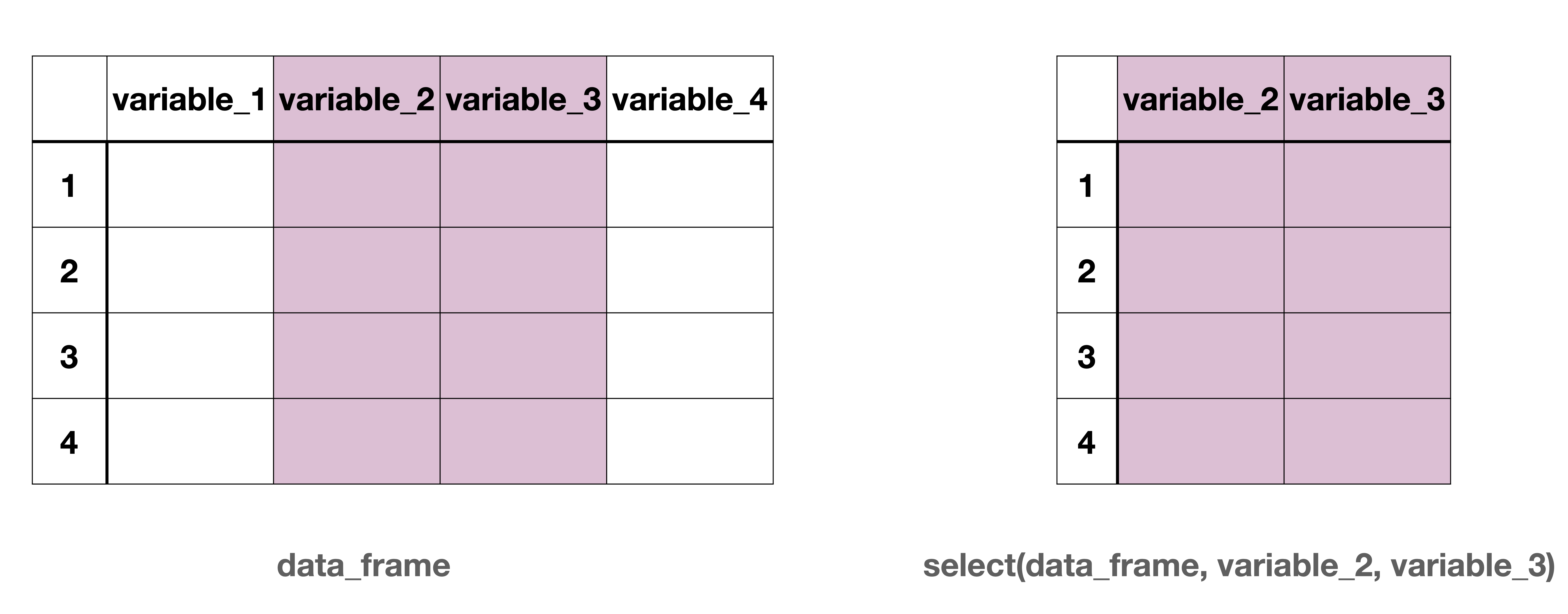
Column-wise subsetting can be done using select().

subsetting observations/rows

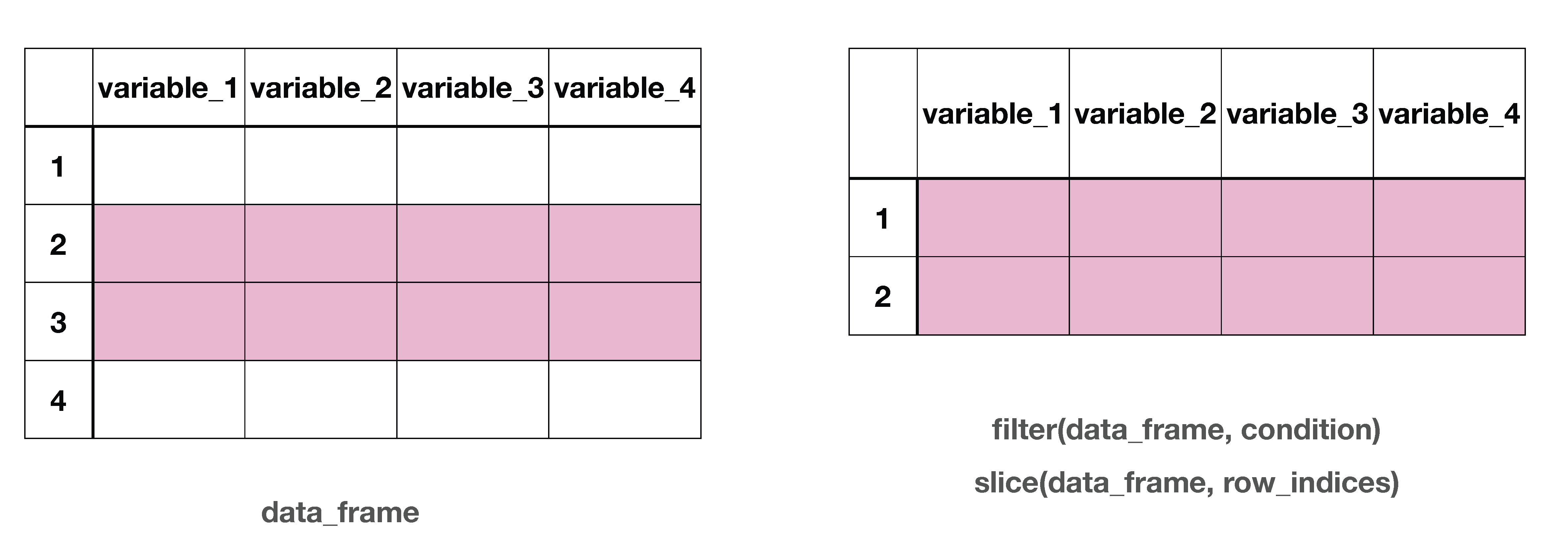
Row-wise subsetting can be done with slice() and filter()

`select()`

select() is used to select certain variables in the data frame.

select(lapd, year, base_pay)

# A tibble: 68,564 × 2
    year base_pay
   <dbl>    <dbl>
 1  2013  105765.
 2  2013   47662.
 3  2013  101288.
 4  2013  118087.
 5  2013   90322.
 6  2013   62770.
 7  2013   93718.
 8  2013       0 
 9  2013   51246.
10  2013   74227.
# ℹ 68,554 more rows

lapd |> 
  select(year, base_pay)

# A tibble: 68,564 × 2
    year base_pay
   <dbl>    <dbl>
 1  2013  105765.
 2  2013   47662.
 3  2013  101288.
 4  2013  118087.
 5  2013   90322.
 6  2013   62770.
 7  2013   93718.
 8  2013       0 
 9  2013   51246.
10  2013   74227.
# ℹ 68,554 more rows

`select()`

select() can also be used to drop certain variables if used with a negative sign.

select(lapd, -row_id, -department_title)

# A tibble: 68,564 × 33
    year payroll_department record_number job_class_title        employment_type
   <dbl>              <dbl>         <dbl> <chr>                  <chr>          
 1  2013               4301    1000027830 Police Detective II    Full Time      
 2  2013               4302    1000155488 Clerk Typist           Full Time      
 3  2013               4301    1000194958 Police Sergeant I      Full Time      
 4  2013               4301    1000232317 Police Lieutenant I    Full Time      
 5  2013               4302    1000329284 Principal Storekeeper  Full Time      
 6  2013               4302    1001124320 Police Service Repres… Full Time      
 7  2013               4301    1001221822 Police Officer III     Full Time      
 8  2013               4301    1001243583 Police Sergeant I      Full Time      
 9  2013               4301    1001317832 Police Officer II      Full Time      
10  2013               4301     100162910 Police Officer II      Full Time      
# ℹ 68,554 more rows
# ℹ 28 more variables: hourly_or_event_rate <dbl>,
#   projected_annual_salary <dbl>, q1_payments <dbl>, q2_payments <dbl>,
#   q3_payments <dbl>, q4_payments <dbl>, payments_over_base_pay <dbl>,
#   percent_over_base_pay <dbl>, total_payments <dbl>, base_pay <dbl>,
#   permanent_bonus_pay <dbl>, longevity_bonus_pay <dbl>,
#   temporary_bonus_pay <dbl>, lump_sum_pay <dbl>, overtime_pay <dbl>, …

Selection helpers

starts_with()
ends_with()
contains()

`starts_with)`

select(lapd, starts_with("q"))

# A tibble: 68,564 × 4
   q1_payments q2_payments q3_payments q4_payments
         <dbl>       <dbl>       <dbl>       <dbl>
 1      24931.      29182.      26546.      29605.
 2      11344.      13212.      11508.      13443.
 3      24184       28327.      28744.      33225.
 4      29391.      36591.      32905.      37234.
 5      20813       24136       21518.      25231.
 6      16057.      17927.      14150.      17052.
 7      22162.      25664.      23404.      24586.
 8          0           0         331.          0 
 9      11941.      14330.      13404.      14537.
10      17046.      20457.      18777.      21371.
# ℹ 68,554 more rows

`ends_with()`

select(lapd, ends_with("pay"))

# A tibble: 68,564 × 8
   payments_over_base_pay percent_over_base_pay base_pay permanent_bonus_pay
                    <dbl>                 <dbl>    <dbl>               <dbl>
 1                  4499.                     0  105765.               3174.
 2                  1845.                     0   47662.                  0 
 3                 13192.                     0  101288.               7364.
 4                 18035.                     0  118087.               7087.
 5                  1376.                     0   90322.                  0 
 6                  2415.                     0   62770.                  0 
 7                  2099.                     0   93718.                866.
 8                   331.                     0       0                   0 
 9                  2967.                     0   51246.               1540.
10                  3424.                     0   74227.               2233.
# ℹ 68,554 more rows
# ℹ 4 more variables: longevity_bonus_pay <dbl>, temporary_bonus_pay <dbl>,
#   lump_sum_pay <dbl>, overtime_pay <dbl>

`contains()`

select(lapd, contains("pay"))

# A tibble: 68,564 × 17
   payroll_department q1_payments q2_payments q3_payments q4_payments
                <dbl>       <dbl>       <dbl>       <dbl>       <dbl>
 1               4301      24931.      29182.      26546.      29605.
 2               4302      11344.      13212.      11508.      13443.
 3               4301      24184       28327.      28744.      33225.
 4               4301      29391.      36591.      32905.      37234.
 5               4302      20813       24136       21518.      25231.
 6               4302      16057.      17927.      14150.      17052.
 7               4301      22162.      25664.      23404.      24586.
 8               4301          0           0         331.          0 
 9               4301      11941.      14330.      13404.      14537.
10               4301      17046.      20457.      18777.      21371.
# ℹ 68,554 more rows
# ℹ 12 more variables: payments_over_base_pay <dbl>,
#   percent_over_base_pay <dbl>, total_payments <dbl>, base_pay <dbl>,
#   permanent_bonus_pay <dbl>, longevity_bonus_pay <dbl>,
#   temporary_bonus_pay <dbl>, lump_sum_pay <dbl>, overtime_pay <dbl>,
#   other_pay_adjustments <dbl>, other_pay_payroll_explorer <dbl>,
#   pay_grade <chr>

`slice()`

slice() subsets rows based on a row number.

The data below include all the rows from third to seventh, including the third and the seventh.

slice(lapd, 3:7)

# A tibble: 5 × 35
  row_id  year department_title payroll_department record_number job_class_title
  <chr>  <dbl> <chr>                         <dbl>         <dbl> <chr>          
1 3-100…  2013 Police (LAPD)                  4301    1000194958 Police Sergean…
2 3-100…  2013 Police (LAPD)                  4301    1000232317 Police Lieuten…
3 3-100…  2013 Police (LAPD)                  4302    1000329284 Principal Stor…
4 3-100…  2013 Police (LAPD)                  4302    1001124320 Police Service…
5 3-100…  2013 Police (LAPD)                  4301    1001221822 Police Officer…
# ℹ 29 more variables: employment_type <chr>, hourly_or_event_rate <dbl>,
#   projected_annual_salary <dbl>, q1_payments <dbl>, q2_payments <dbl>,
#   q3_payments <dbl>, q4_payments <dbl>, payments_over_base_pay <dbl>,
#   percent_over_base_pay <dbl>, total_payments <dbl>, base_pay <dbl>,
#   permanent_bonus_pay <dbl>, longevity_bonus_pay <dbl>,
#   temporary_bonus_pay <dbl>, lump_sum_pay <dbl>, overtime_pay <dbl>,
#   other_pay_adjustments <dbl>, other_pay_payroll_explorer <dbl>, mou <chr>, …

Relational and Logical Operators

Operator	Description
<	Less than
>	Greater than
<=	Less than or equal to
>=	Greater than or equal to
==	Equal to
!=	Not equal to

Operator	Description
&	and
\|	or

`filter()`

filter() subsets rows based on a condition.

The data below includes rows when the recorded year is 2018.

filter(lapd, year == 2018)

# A tibble: 14,824 × 35
   row_id            year department_title payroll_department record_number
   <chr>            <dbl> <chr>                         <dbl>         <dbl>
 1 8-1000027830ctFu  2018 Police (LAPD)                  4301    1000027830
 2 8-1000194958ctFu  2018 Police (LAPD)                  4301    1000194958
 3 8-1000232317ctFu  2018 Police (LAPD)                  4301    1000232317
 4 8-1001124320ctFu  2018 Police (LAPD)                  4302    1001124320
 5 8-1001221822ctFu  2018 Police (LAPD)                  4301    1001221822
 6 8-1001317832ctFu  2018 Police (LAPD)                  4301    1001317832
 7 8-100162910ctFu   2018 Police (LAPD)                  4301     100162910
 8 8-1001675957ctFu  2018 Police (LAPD)                  4301    1001675957
 9 8-1001884819ctFu  2018 Police (LAPD)                  4302    1001884819
10 8-1001893163ctFu  2018 Police (LAPD)                  4302    1001893163
# ℹ 14,814 more rows
# ℹ 30 more variables: job_class_title <chr>, employment_type <chr>,
#   hourly_or_event_rate <dbl>, projected_annual_salary <dbl>,
#   q1_payments <dbl>, q2_payments <dbl>, q3_payments <dbl>, q4_payments <dbl>,
#   payments_over_base_pay <dbl>, percent_over_base_pay <dbl>,
#   total_payments <dbl>, base_pay <dbl>, permanent_bonus_pay <dbl>,
#   longevity_bonus_pay <dbl>, temporary_bonus_pay <dbl>, lump_sum_pay <dbl>, …

Example 1

Q. How many LAPD staff members had a base pay higher than $100,000 in year 2018 according to this data?

Example 1

lapd |> 
  filter(year == 2018 & base_pay > 100000)

# A tibble: 6,499 × 35
   row_id            year department_title payroll_department record_number
   <chr>            <dbl> <chr>                         <dbl>         <dbl>
 1 8-1000027830ctFu  2018 Police (LAPD)                  4301    1000027830
 2 8-1000194958ctFu  2018 Police (LAPD)                  4301    1000194958
 3 8-1000232317ctFu  2018 Police (LAPD)                  4301    1000232317
 4 8-1001221822ctFu  2018 Police (LAPD)                  4301    1001221822
 5 8-1001945123ctFu  2018 Police (LAPD)                  4301    1001945123
 6 8-1002130218ctFu  2018 Police (LAPD)                  4301    1002130218
 7 8-1002409510ctFu  2018 Police (LAPD)                  4301    1002409510
 8 8-100305817ctFu   2018 Police (LAPD)                  4302     100305817
 9 8-100309798ctFu   2018 Police (LAPD)                  4301     100309798
10 8-1003303056ctFu  2018 Police (LAPD)                  4301    1003303056
# ℹ 6,489 more rows
# ℹ 30 more variables: job_class_title <chr>, employment_type <chr>,
#   hourly_or_event_rate <dbl>, projected_annual_salary <dbl>,
#   q1_payments <dbl>, q2_payments <dbl>, q3_payments <dbl>, q4_payments <dbl>,
#   payments_over_base_pay <dbl>, percent_over_base_pay <dbl>,
#   total_payments <dbl>, base_pay <dbl>, permanent_bonus_pay <dbl>,
#   longevity_bonus_pay <dbl>, temporary_bonus_pay <dbl>, lump_sum_pay <dbl>, …

Example 1

lapd |> 
  filter(year == 2018 & base_pay > 100000) |> 
  nrow()

[1] 6499

Example 2

Q. How many observations are available between 2013 and 2015 including 2013 and 2015?

lapd |> 
  filter(year >= 2013 & year <= 2015)

# A tibble: 40,227 × 35
   row_id            year department_title payroll_department record_number
   <chr>            <dbl> <chr>                         <dbl>         <dbl>
 1 3-1000027830ctFu  2013 Police (LAPD)                  4301    1000027830
 2 3-1000155488ctFu  2013 Police (LAPD)                  4302    1000155488
 3 3-1000194958ctFu  2013 Police (LAPD)                  4301    1000194958
 4 3-1000232317ctFu  2013 Police (LAPD)                  4301    1000232317
 5 3-1000329284ctFu  2013 Police (LAPD)                  4302    1000329284
 6 3-1001124320ctFu  2013 Police (LAPD)                  4302    1001124320
 7 3-1001221822ctFu  2013 Police (LAPD)                  4301    1001221822
 8 3-1001243583ctFu  2013 Police (LAPD)                  4301    1001243583
 9 3-1001317832ctFu  2013 Police (LAPD)                  4301    1001317832
10 3-100162910ctFu   2013 Police (LAPD)                  4301     100162910
# ℹ 40,217 more rows
# ℹ 30 more variables: job_class_title <chr>, employment_type <chr>,
#   hourly_or_event_rate <dbl>, projected_annual_salary <dbl>,
#   q1_payments <dbl>, q2_payments <dbl>, q3_payments <dbl>, q4_payments <dbl>,
#   payments_over_base_pay <dbl>, percent_over_base_pay <dbl>,
#   total_payments <dbl>, base_pay <dbl>, permanent_bonus_pay <dbl>,
#   longevity_bonus_pay <dbl>, temporary_bonus_pay <dbl>, lump_sum_pay <dbl>, …

Example 2

lapd |> 
  filter(year >= 2013 & year <= 2015) |> 
  nrow()

[1] 40227

Example 3

Q. How many LAPD staff were employed full time in 2018?

lapd |> 
  filter(employment_type == "Full Time" & year == 2018) |> 
  nrow()

[1] 14664

Data frame is unchanged

We have done all sorts of selections, slicing, filtering on lapd but it has not changed at all. Why do you think so?

glimpse(lapd)

Rows: 68,564
Columns: 35
$ row_id                     <chr> "3-1000027830ctFu", "3-1000155488ctFu", "3-…
$ year                       <dbl> 2013, 2013, 2013, 2013, 2013, 2013, 2013, 2…
$ department_title           <chr> "Police (LAPD)", "Police (LAPD)", "Police (…
$ payroll_department         <dbl> 4301, 4302, 4301, 4301, 4302, 4302, 4301, 4…
$ record_number              <dbl> 1000027830, 1000155488, 1000194958, 1000232…
$ job_class_title            <chr> "Police Detective II", "Clerk Typist", "Pol…
$ employment_type            <chr> "Full Time", "Full Time", "Full Time", "Ful…
$ hourly_or_event_rate       <dbl> 53.16, 23.77, 60.80, 60.98, 45.06, 34.42, 4…
$ projected_annual_salary    <dbl> 110998.08, 49623.67, 126950.40, 127326.24, …
$ q1_payments                <dbl> 24931.20, 11343.96, 24184.00, 29391.20, 208…
$ q2_payments                <dbl> 29181.61, 13212.37, 28327.20, 36591.20, 241…
$ q3_payments                <dbl> 26545.80, 11508.36, 28744.20, 32904.81, 215…
$ q4_payments                <dbl> 29605.30, 13442.53, 33224.88, 37234.03, 252…
$ payments_over_base_pay     <dbl> 4499.12, 1844.82, 13192.43, 18034.53, 1376.…
$ percent_over_base_pay      <dbl> 0, 0, 0, 0, 0, 0, 0, 0, 0, 0, 0, 0, 0, 0, 0…
$ total_payments             <dbl> 110263.91, 49507.22, 114480.28, 136121.24, …
$ base_pay                   <dbl> 105764.79, 47662.40, 101287.85, 118086.71, …
$ permanent_bonus_pay        <dbl> 3174.12, 0.00, 7363.95, 7086.67, 0.00, 0.00…
$ longevity_bonus_pay        <dbl> 0.00, 1310.82, 0.00, 0.00, 1251.19, 1726.16…
$ temporary_bonus_pay        <dbl> 1325.00, 0.00, 1205.00, 1325.00, 125.00, 68…
$ lump_sum_pay               <dbl> 0.00, 0.00, 2133.18, 0.00, 2068.80, 0.00, 0…
$ overtime_pay               <dbl> 0.00, 0.00, 4424.32, 9839.33, 0.00, 0.00, 4…
$ other_pay_adjustments      <dbl> 0.00, 534.00, -1934.02, -216.47, -2068.80, …
$ other_pay_payroll_explorer <dbl> 4499.12, 1844.82, 8768.11, 8195.20, 1376.19…
$ mou                        <chr> "24", "3", "24", "24", "12", "3", "24", "24…
$ mou_title                  <chr> "POLICE OFFICERS UNIT", "CLERICAL UNIT", "P…
$ fms_department             <dbl> 70, 70, 70, 70, 70, 70, 70, 70, 70, 70, 70,…
$ job_class                  <chr> "2223", "1358", "2227", "2232", "1839", "22…
$ pay_grade                  <chr> "2", "0", "1", "1", "0", "2", "3", "1", "B"…
$ average_health_cost        <dbl> 11651.40, 10710.24, 11651.40, 11651.40, 107…
$ average_dental_cost        <dbl> 898.08, 405.24, 898.08, 898.08, 405.24, 405…
$ average_basic_life         <dbl> 191.04, 11.40, 191.04, 191.04, 11.40, 11.40…
$ average_benefit_cost       <dbl> 12740.52, 11126.88, 12740.52, 12740.52, 111…
$ benefits_plan              <chr> "Police", "City", "Police", "Police", "City…
$ job_class_link             <chr> "http://per.lacity.org/perspecs/2223.pdf", …

Moving forward

Moving forward we are only going to focus on year 2018, and use job_class_title, employment_type, and base_pay. Let’s clean our data accordingly and move on with the smaller lapd data that we need.

Moving forward

lapd |> 
  filter(year == 2018) |> 
  select(job_class_title, employment_type, base_pay)

# A tibble: 14,824 × 3
   job_class_title                  employment_type base_pay
   <chr>                            <chr>              <dbl>
 1 Police Detective II              Full Time        119322.
 2 Police Sergeant I                Full Time        113271.
 3 Police Lieutenant II             Full Time        148116 
 4 Police Service Representative II Full Time         78677.
 5 Police Officer III               Full Time        109374.
 6 Police Officer II                Full Time         95002.
 7 Police Officer II                Full Time         95379.
 8 Police Officer II                Full Time         95388.
 9 Equipment Mechanic               Full Time         80496 
10 Detention Officer                Full Time         69640 
# ℹ 14,814 more rows

Moving forward

lapd <- 
  lapd |> 
  filter(year == 2018) |> 
  select(job_class_title, employment_type, base_pay)

Moving forward

glimpse(lapd)

Rows: 14,824
Columns: 3
$ job_class_title <chr> "Police Detective II", "Police Sergeant I", "Police Li…
$ employment_type <chr> "Full Time", "Full Time", "Full Time", "Full Time", "F…
$ base_pay        <dbl> 119321.60, 113270.70, 148116.00, 78676.87, 109373.63, …

Changing Variables

Goal

Create a new variable called base_pay_k that represents base_pay in thousand dollars.

`mutate()`

lapd |> 
  mutate(base_pay_k = base_pay/1000)

# A tibble: 14,824 × 4
   job_class_title                  employment_type base_pay base_pay_k
   <chr>                            <chr>              <dbl>      <dbl>
 1 Police Detective II              Full Time        119322.      119. 
 2 Police Sergeant I                Full Time        113271.      113. 
 3 Police Lieutenant II             Full Time        148116       148. 
 4 Police Service Representative II Full Time         78677.       78.7
 5 Police Officer III               Full Time        109374.      109. 
 6 Police Officer II                Full Time         95002.       95.0
 7 Police Officer II                Full Time         95379.       95.4
 8 Police Officer II                Full Time         95388.       95.4
 9 Equipment Mechanic               Full Time         80496        80.5
10 Detention Officer                Full Time         69640        69.6
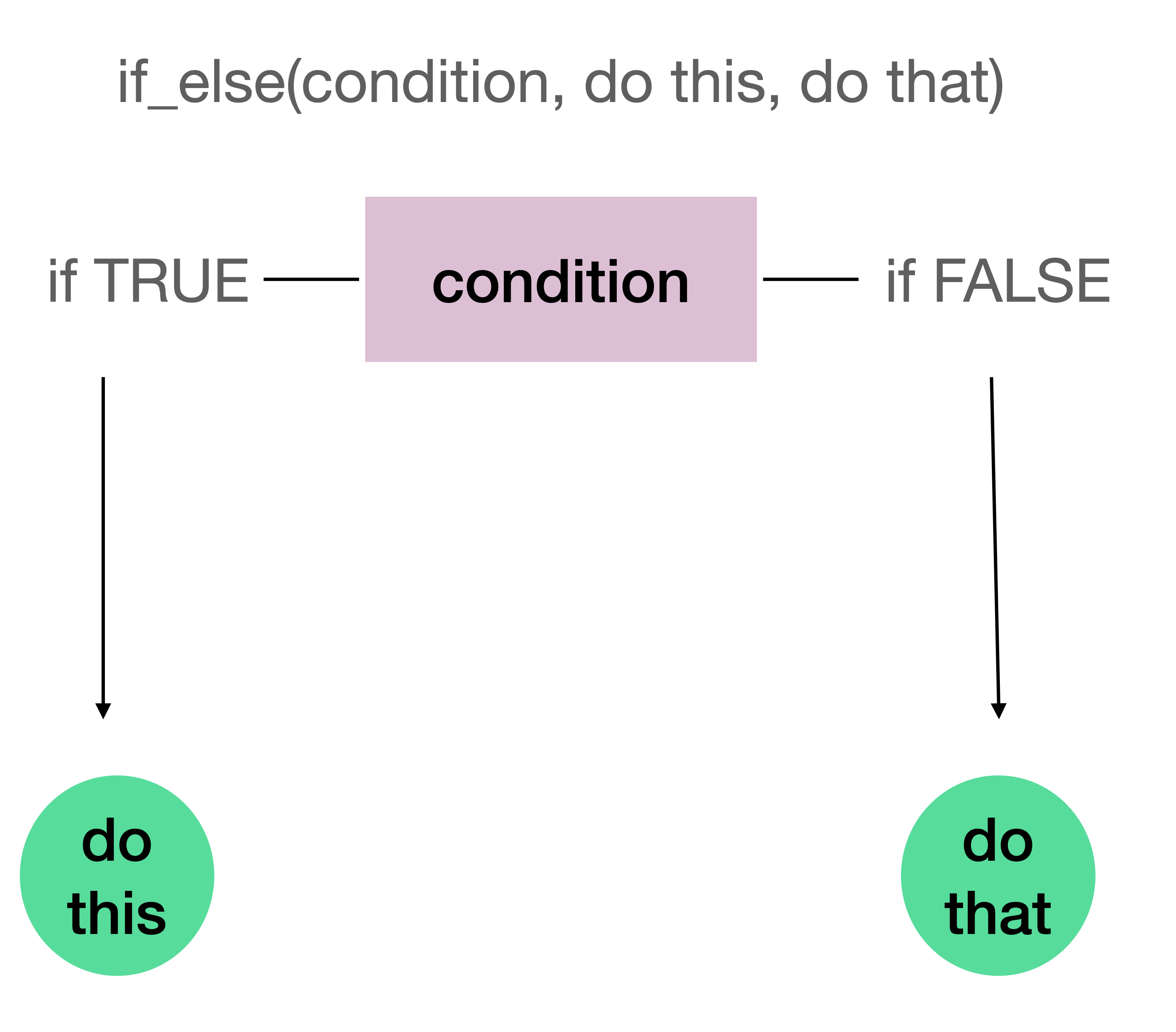
# ℹ 14,814 more rows

Goal

Create a new variable called base_pay_class which has two classifications: “Less than 100K”, “More than 100K”.

Side question

Let’s first check to see there is anyone earning exactly 100K.

lapd |> 
  filter(base_pay == 100000)

# A tibble: 0 × 3
# ℹ 3 variables: job_class_title <chr>, employment_type <chr>, base_pay <dbl>

`if_else()`

lapd |> 
  mutate(
    base_pay_class = if_else(
      base_pay < 100000, "Less than 100K", "More than 100K"
    )
  )

# A tibble: 14,824 × 4
   job_class_title                  employment_type base_pay base_pay_class
   <chr>                            <chr>              <dbl> <chr>         
 1 Police Detective II              Full Time        119322. More than 100K
 2 Police Sergeant I                Full Time        113271. More than 100K
 3 Police Lieutenant II             Full Time        148116  More than 100K
 4 Police Service Representative II Full Time         78677. Less than 100K
 5 Police Officer III               Full Time        109374. More than 100K
 6 Police Officer II                Full Time         95002. Less than 100K
 7 Police Officer II                Full Time         95379. Less than 100K
 8 Police Officer II                Full Time         95388. Less than 100K
 9 Equipment Mechanic               Full Time         80496  Less than 100K
10 Detention Officer                Full Time         69640  Less than 100K
# ℹ 14,814 more rows

`if_else()` summary

Flowchart illustrating an if–else decision. At the top is the text if_else(condition, do this, do that). A central pink rectangle labeled condition branches into two paths: to the left, labeled if TRUE, an arrow points down to a green circle labeled do this; to the right, labeled if FALSE, an arrow points down to a green circle labeled do that. The diagram shows how a condition determines which action is executed.

Figure 1

Goal

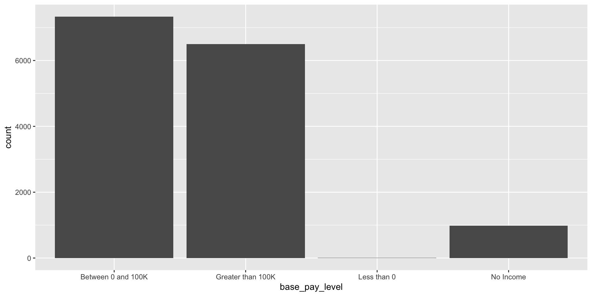
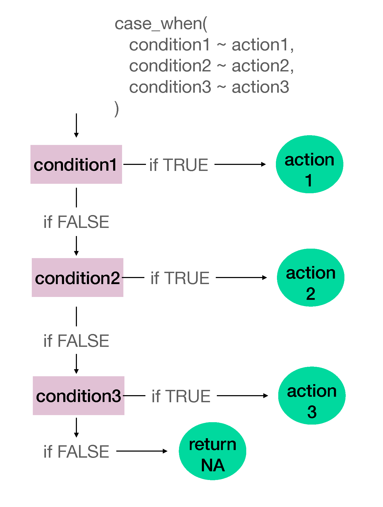
Create a new variable called base_pay_level which has Less Than 0, No Income, Between 0 and 100K and Greater than 100K.

`case_when()`

lapd |> 
  mutate(
    base_pay_level = case_when(
      base_pay < 0 ~ "Less than 0", 
      base_pay == 0 ~ "No Income",
      base_pay < 100000 & base_pay > 0 ~ "Between 0 and 100K",
      base_pay > 100000 ~ "Greater than 100K"
    )
  )

# A tibble: 14,824 × 4
   job_class_title                  employment_type base_pay base_pay_level    
   <chr>                            <chr>              <dbl> <chr>             
 1 Police Detective II              Full Time        119322. Greater than 100K 
 2 Police Sergeant I                Full Time        113271. Greater than 100K 
 3 Police Lieutenant II             Full Time        148116  Greater than 100K 
 4 Police Service Representative II Full Time         78677. Between 0 and 100K
 5 Police Officer III               Full Time        109374. Greater than 100K 
 6 Police Officer II                Full Time         95002. Between 0 and 100K
 7 Police Officer II                Full Time         95379. Between 0 and 100K
 8 Police Officer II                Full Time         95388. Between 0 and 100K
 9 Equipment Mechanic               Full Time         80496  Between 0 and 100K
10 Detention Officer                Full Time         69640  Between 0 and 100K
# ℹ 14,814 more rows

Pipes

We can use pipes with ggplot too!

lapd |> 
  mutate(base_pay_level = case_when(
    base_pay < 0 ~ "Less than 0", 
    base_pay == 0 ~ "No Income",
    base_pay < 100000 & base_pay > 0 ~ "Between 0 and 100K",
    base_pay > 100000 ~ "Greater than 100K")) |> 
  ggplot(aes(x = base_pay_level)) +
  geom_bar()

a var plot of base_pay_level showing the newly created levels as Between 0 and 100K, Greater than 100K, Less than 0, and No Income

`case_when()` summary

Flowchart illustrating case_when logic. At the top is the text case_when(condition1 ~ action1, condition2 ~ action2, condition3 ~ action3). A vertical sequence of pink rectangles labeled condition1, condition2, and condition3 represents conditions evaluated in order. For each condition, a rightward arrow labeled if TRUE leads to a green circle labeled action1, action2, or action3, respectively. If a condition is false, the flow continues downward to the next condition. If all conditions are false, a final arrow leads to a green circle labeled return NA. The diagram shows how the first true condition determines the returned action.

Figure 2

Goal

Make job_class_title and employment_type factor variables.

`as.factor()`

lapd |> 
  mutate(
    employment_type = as.factor(employment_type),
    job_class_title = as.factor(job_class_title)
  )

# A tibble: 14,824 × 3
   job_class_title                  employment_type base_pay
   <fct>                            <fct>              <dbl>
 1 Police Detective II              Full Time        119322.
 2 Police Sergeant I                Full Time        113271.
 3 Police Lieutenant II             Full Time        148116 
 4 Police Service Representative II Full Time         78677.
 5 Police Officer III               Full Time        109374.
 6 Police Officer II                Full Time         95002.
 7 Police Officer II                Full Time         95379.
 8 Police Officer II                Full Time         95388.
 9 Equipment Mechanic               Full Time         80496 
10 Detention Officer                Full Time         69640 
# ℹ 14,814 more rows

Changing variable types

as.factor() - makes a vector factor
as.numeric() - makes a vector numeric
as.integer() - makes a vector integer
as.double() - makes a vector double
as.character() - makes a vector character

Writing data

Once again we did not “save” anything into lapd. As we work on data cleaning it makes sense not to “save” the data frames. Once we see the final data frame we want then we can “save” (i.e. overwrite) it.

In your lecture notes, you can do all the changes in this lecture in one long set of piped code. That’s the beauty of piping!

Cleaning in one long chain

lapd <- 
  lapd |> 
  clean_names() |> 
  filter(year == 2018) |> 
  select(job_class_title, employment_type, base_pay) |> 
  mutate(
    employment_type = as.factor(employment_type),
    job_class_title = as.factor(job_class_title),
    base_pay_class = if_else(
      base_pay < 100000, "Less than 100K", "More than 100K"
    ),
    base_pay_level = case_when(
      base_pay < 0 ~ "Less than 0", 
      base_pay == 0 ~ "No Income",
      base_pay < 100000 & base_pay > 0 ~ "Between 0 and 100K",
      base_pay > 100000 ~ "Greater than 100K"
    )
  )

Pay attention to first argument

Warning

The functions clean_names(), select(), filter(), mutate() all take a data frame as the first argument. Even though we do not see it, the data frame is piped through from the previous step of code at each step. When we use these functions without the |> we have to include the data frame explicitly.

Data frame is used as the first argument

clean_names(lapd)

Data frame is piped

lapd |> 
  clean_names()

Learning Tip of the Day

Exercise Improves Academic Performance

Data Wrangling Part I

Three solutions to a single problem

Breaking down the question

Solution 1: Functions within Functions

Problem!

Solution 2: Creating Objects

Problem!

Solution 3: The (forward) Pipe Operator |>

RStudio settings

Reading the pipe operator

Recall functions from algebra

Data

Tidy style names

Subsetting Data Frames

subsetting variables/columns

subsetting observations/rows

select()

select()

Selection helpers

starts_with)

ends_with()

contains()

slice()

Relational and Logical Operators

filter()

Example 1

Example 1

Example 1

Example 2

Example 2

Example 3

Data frame is unchanged

Moving forward

Moving forward

Moving forward

Moving forward

Changing Variables

Goal

mutate()

Goal

Side question

if_else()

if_else() summary

Goal

case_when()

Pipes

case_when() summary

Goal

as.factor()

Changing variable types

Writing data

Cleaning in one long chain

Pay attention to first argument

Learning Tip of the Day

Data Wrangling
Part I

`select()`

`select()`

`starts_with)`

`ends_with()`

`contains()`

`slice()`

`filter()`

`mutate()`

`if_else()`

`if_else()` summary

`case_when()`

`case_when()` summary

`as.factor()`