- 1
- We will use the stringr package for handling strings.
- 2
- We will use the lubridate package for handling dates.
- 3
- We will use the forcats package for handling factors. You can think of forcats as for cat egorical variable s or as an anagram of factors.
Working with Strings, Dates, and Factors
Dr. Mine Dogucu
Packages
Packages
All these packages are part of tidyverse
── Attaching core tidyverse packages ──────────────────────── tidyverse 2.0.0 ──
✔ dplyr   1.2.1     ✔ readr   2.2.0
✔ ggplot2 4.0.2     ✔ tibble  3.3.1
✔ purrr   1.2.2     ✔ tidyr   1.3.2
── Conflicts ────────────────────────────────────────── tidyverse_conflicts() ──
✖ dplyr::filter() masks stats::filter()
✖ dplyr::lag()    masks stats::lag()
ℹ Use the conflicted package (<http://conflicted.r-lib.org/>) to force all conflicts to become errors
Data
glimpse
Rows: 369,089
Columns: 36
$ call_number                    <dbl> 250010495, 250010101, 250010606, 250010…
$ unit_id                        <chr> "T06", "T07", "B01", "E03", "M555", "B0…
$ incident_number                <dbl> 25000102, 25000013, 25000123, 25000084,…
$ call_type                      <chr> "Alarms", "Alarms", "Alarms", "Traffic …
$ call_date                      <chr> "01/01/2025", "01/01/2025", "01/01/2025…
$ watch_date                     <chr> "12/31/2024", "12/31/2024", "12/31/2024…
$ received_dt_tm                 <chr> "2025 Jan 01 02:18:24 AM", "2025 Jan 01…
$ entry_dt_tm                    <chr> "2025 Jan 01 02:19:59 AM", "2025 Jan 01…
$ dispatch_dt_tm                 <chr> "2025 Jan 01 02:21:00 AM", "2025 Jan 01…
$ response_dt_tm                 <chr> "2025 Jan 01 02:23:46 AM", "2025 Jan 01…
$ on_scene_dt_tm                 <chr> "2025 Jan 01 02:28:33 AM", "2025 Jan 01…
$ transport_dt_tm                <chr> NA, NA, NA, NA, "2025 Jan 01 01:33:03 A…
$ hospital_dt_tm                 <chr> NA, NA, NA, NA, "2025 Jan 01 01:44:31 A…
$ call_final_disposition         <chr> "Fire", "Fire", "Fire", "Code 2 Transpo…
$ available_dt_tm                <chr> "2025 Jan 01 02:30:48 AM", "2025 Jan 01…
$ address                        <chr> "18TH ST/MARKET ST", "19TH ST/MISSION S…
$ city                           <chr> "San Francisco", "San Francisco", "San …
$ zipcode_of_incident            <dbl> 94114, 94110, 94108, 94102, 94107, 9412…
$ battalion                      <chr> "B05", "B02", "B01", "B02", "B03", "B07…
$ station_area                   <chr> "24", "07", "13", "36", "08", "14", "36…
$ box                            <chr> "5413", "5423", "1313", "1552", "2154",…
$ original_priority              <chr> "3", "3", NA, "A", "3", "3", "3", "3", …
$ priority                       <chr> "3", "3", "3", "3", "3", "3", "3", "3",…
$ final_priority                 <dbl> 3, 3, 3, 3, 3, 3, 3, 3, 3, 3, 3, 3, 2, …
$ als_unit                       <lgl> FALSE, FALSE, FALSE, FALSE, TRUE, FALSE…
$ call_type_group                <chr> "Alarm", "Alarm", "Alarm", "Non Life-th…
$ number_of_alarms               <dbl> 1, 1, 1, 1, 1, 1, 1, 1, 1, 1, 1, 1, 1, …
$ unit_type                      <chr> "TRUCK", "TRUCK", "CHIEF", "ENGINE", "M…
$ unit_sequence_in_call_dispatch <dbl> 2, 3, 2, 1, 1, 2, 1, 1, 3, 3, 10, 2, 3,…
$ fire_prevention_district       <chr> "5", "6", "1", "2", "3", "7", "2", "2",…
$ supervisor_district            <dbl> 8, 9, 3, 5, 6, 1, 6, 5, 6, 5, 5, 2, 5, …
$ neighborhoods_boundaries       <chr> "Castro/Upper Market", "Mission", "Chin…
$ row_id                         <chr> "250010495-T06", "250010101-T07", "2500…
$ case_location                  <chr> "POINT (-122.444629428 37.759708374)", …
$ data_as_of                     <chr> "2025 Jan 01 03:32:04 AM", "2025 Jan 01…
$ data_loaded_at                 <chr> "2025 Jan 08 04:18:30 AM", "2025 Jan 08…
Strings
Replace a string
Replace a string
# A tibble: 369,089 × 1
   address_long
   <chr>
 1 18TH STREET/MARKET STREET
 2 19TH STREET/MISSION STREET
 3 CLAY STREET/GRANT AVE
 4 FULTON STREET/HYDE STREET/UNITED NATIONS PLZ
 5 02ND STREET/KING STREET
 6 31STREET AVE/FULTON STREET
 7 09TH STREET/JESSIE STREET
 8 POLK STREET/WILLOW STREET
 9 06TH STREET/STREETEVENSON STREET
10 GEARY STREET/JONES STREET
# ℹ 369,079 more rows
Replace a string
Replace a string
# A tibble: 369,089 × 1
   address_long
   <chr>
 1 18TH STREET/MARKET STREET
 2 19TH STREET/MISSION STREET
 3 CLAY STREET/GRANT AVENUE
 4 FULTON STREET/HYDE STREET/UNITED NATIONS PLACEZ
 5 02ND STREET/KING STREET
 6 31STREET AVENUE/FULTON STREET
 7 09TH STREET/JESSIE STREET
 8 POLK STREET/WILLOW STREET
 9 06TH STREET/STREETEVENSON STREET
10 GEARY STREET/JONES STREET
# ℹ 369,079 more rows
Change letter types
# A tibble: 6 × 1
  address
  <chr>
1 18th St/Market St
2 19th St/Mission St
3 Clay St/Grant Ave
4 Fulton St/Hyde St/United Nations Plz
5 02nd St/King St
6 31st Ave/Fulton St
We can also use str_to_upper() or str_to_lower() as needed
glue
# A tibble: 3 × 1
  description
  <glue>
1 Incident 250010495 occurred in Castro/Upper Market
2 Incident 250010101 occurred in Mission
3 Incident 250010606 occurred in Chinatown
detect
# A tibble: 10 × 2
   call_type                          is_fire_related
   <chr>                              <lgl>
 1 Medical Incident                   FALSE
 2 Medical Incident                   FALSE
 3 Structure Fire / Smoke in Building TRUE
 4 Structure Fire / Smoke in Building TRUE
 5 Medical Incident                   FALSE
 6 Structure Fire / Smoke in Building TRUE
 7 Medical Incident                   FALSE
 8 Medical Incident                   FALSE
 9 Medical Incident                   FALSE
10 Medical Incident                   FALSE
Dates
ISO Date
Note
While there are many ways to write a date for humans, there is only one universally accepted format for data as standardized by the International Organization for Standardization (ISO). It follows the order of YYYY-MM-DD (e.g., 1986-12-20). Writing dates this way ensures they are sorted correctly by computers and avoids any international confusion between months and days.
UTC and Timezones
UTC stands for Coordinated Universal Time. Think of it as the world’s main clock.
UTC is not a timezone but a high-precision time standard that all time zones use to stay synchronized.
UTC never observes Daylight Saving Time, it never skips or repeats hours, making it the safest format for storing data and performing math.
Irvine is UTC-8 (8 hours behind UTC) between first Sunday of November and second Sunday of March which is specified as Pacific Standard Time (PST) and UTC-7 during rest of the year which is specified as Pacific Daylight Time (PDT).
received_dt_tm
ymd_hms()
received_dt_tm
with time zone
# A tibble: 3 × 1
  received_dt_tm
  <dttm>
1 2024-12-31 18:18:24
2 2024-12-31 16:20:36
3 2024-12-31 19:00:07
OlsonNames() function lists different names of timezones.
hour, month and week day
# A tibble: 3 × 4
  received_dt_tm      hour_val month_val day_name
  <dttm>                 <int> <ord>     <ord>
1 2024-12-31 18:18:24       18 Dec       Tue
2 2024-12-31 16:20:36       16 Dec       Tue
3 2024-12-31 19:00:07       19 Dec       Tue
duration
# A tibble: 3 × 2
  received_dt_tm      goal_arrival_time
  <dttm>              <dttm>
1 2024-12-31 18:18:24 2024-12-31 18:26:24
2 2024-12-31 16:20:36 2024-12-31 16:28:36
3 2024-12-31 19:00:07 2024-12-31 19:08:07
duration
[1] "2026-03-08 06:00:00 PDT"[1] "2026-03-08 05:00:00 PDT"Note
When performing math with dates, lubridate distinguishes between two ways of measuring time: durations and periods. This distinction is critical when your data spans a Daylight Saving Time (DST) transition. The above example shows a hypothetical event start time as March 7th, 2026 at 5:00 in Los Angeles time zone. When you add duration of exactly 1 day using the ddays() function, you are simply adding 86,400 seconds. When 86,400 seconds have passed the clocks would be showing 06:00 am on March 8th, 2026 due to start of Daylight Saving Time. On the other end, the days() function just adds one day to the calendar day without touching the time component.
difftime
today and now
Factors
as.factor()
levels()
levels() as seen in ggplot
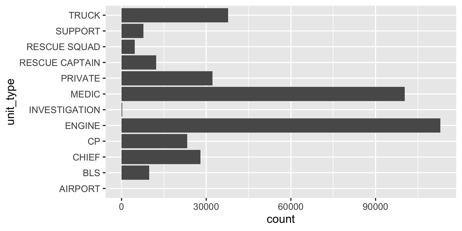
Figure 1
fct_infreq()
levels() as seen in ggplot
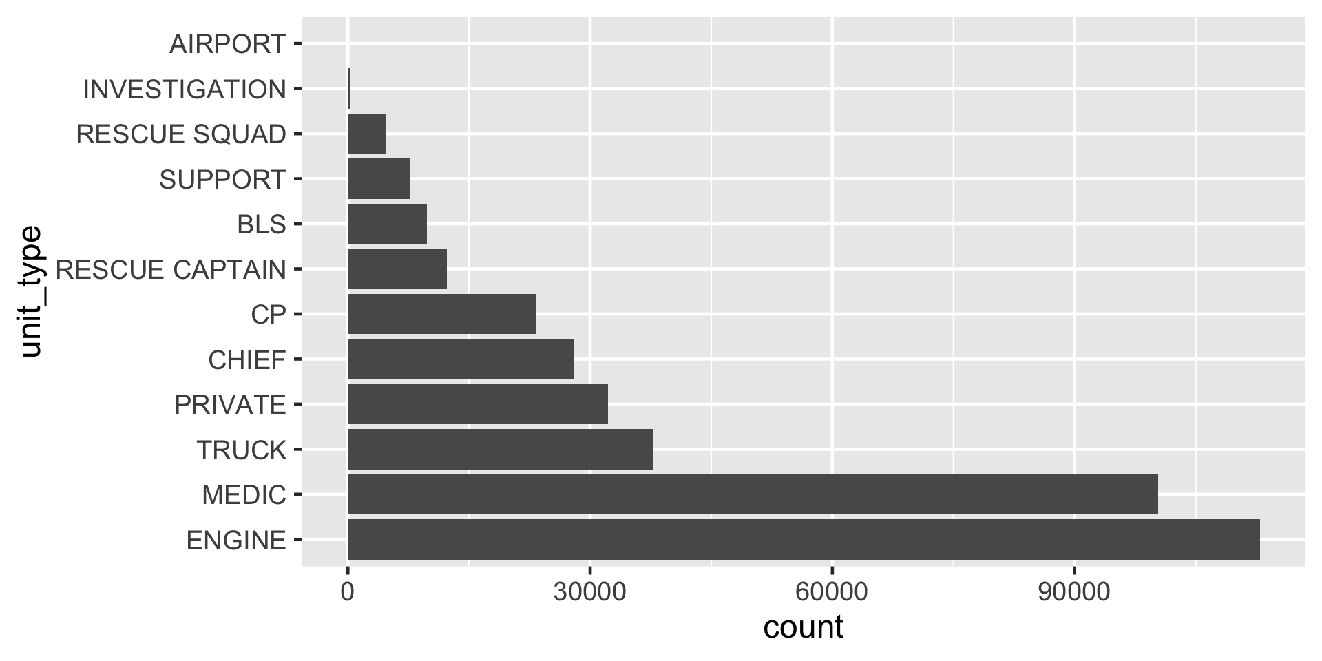
Figure 2
levels() as seen in ggplot with fct_rev()
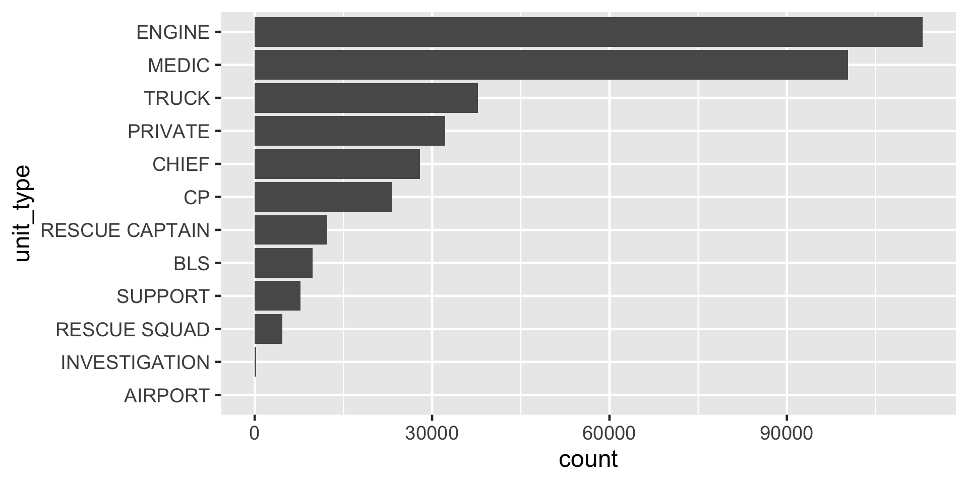
Figure 3
levels() as seen in ggplot with fct_lump_n()
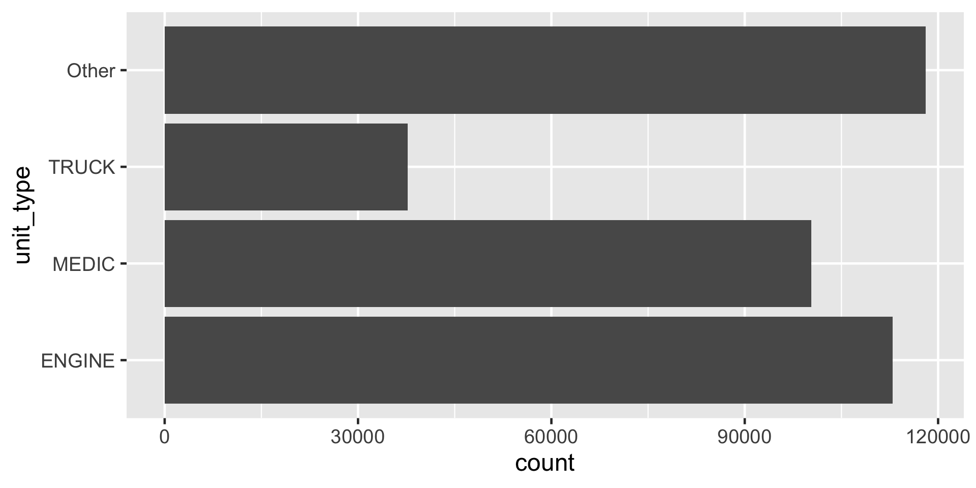
Figure 4
fct_relevel()
# A tibble: 12 × 2
   unit_type      total_als_unit
   <fct>                   <int>
 1 ENGINE                  89853
 2 MEDIC                   88065
 3 TRUCK                    2336
 4 PRIVATE                     0
 5 CHIEF                       0
 6 CP                        135
 7 RESCUE CAPTAIN           9821
 8 BLS                         0
 9 SUPPORT                  5059
10 RESCUE SQUAD                0
11 INVESTIGATION               0
12 AIRPORT                     0
fct_relevel()
# A tibble: 12 × 2
   unit_type      total_als_unit
   <fct>                   <int>
 1 ENGINE                  89853
 2 TRUCK                    2336
 3 MEDIC                   88065
 4 PRIVATE                     0
 5 CHIEF                       0
 6 CP                        135
 7 RESCUE CAPTAIN           9821
 8 BLS                         0
 9 SUPPORT                  5059
10 RESCUE SQUAD                0
11 INVESTIGATION               0
12 AIRPORT                     0
fct_reorder()
 Factor w/ 42 levels "Bayview Hunters Point",..: 3 19 4 37 20 27 35 37 35 37 ...
 Factor w/ 42 levels "Nob Hill","Western Addition",..: 15 10 8 12 22 16 24 12 24 12 ...