library(bayesrules)
library(tidyverse)Introduction to Bayesian Inference:
The Beta-Binomial Model
The Optimist
summarize_beta(14, 1) mean mode var sd
1 0.9333333 1 0.003888889 0.06236096plot_beta(14, 1) 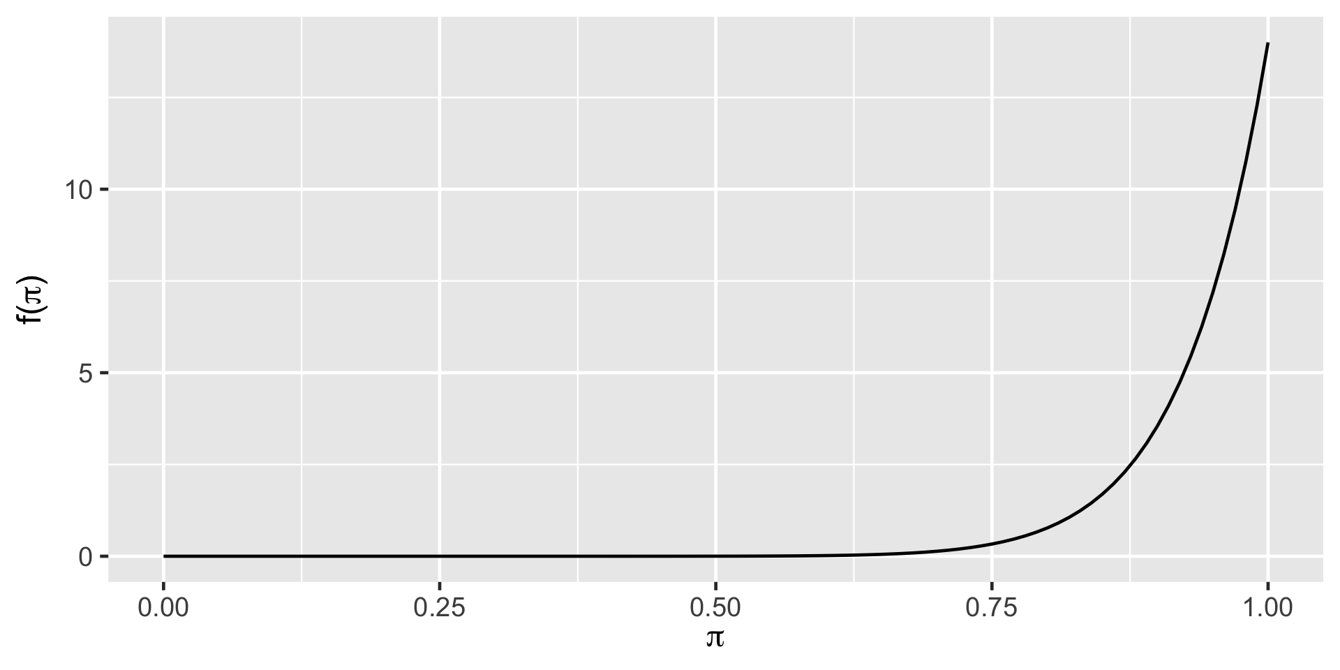
The Clueless
summarize_beta(1, 1) mean mode var sd
1 0.5 NaN 0.08333333 0.2886751plot_beta(1, 1) 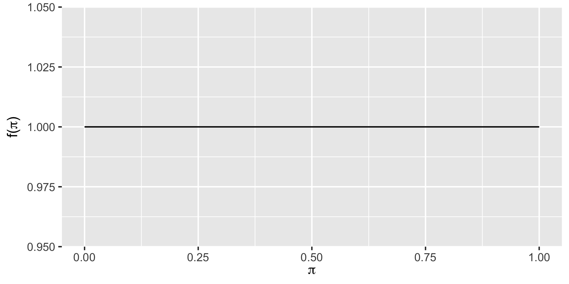
The Feminist
summarize_beta(5, 11) mean mode var sd
1 0.3125 0.2857143 0.01263787 0.1124183plot_beta(5, 11) 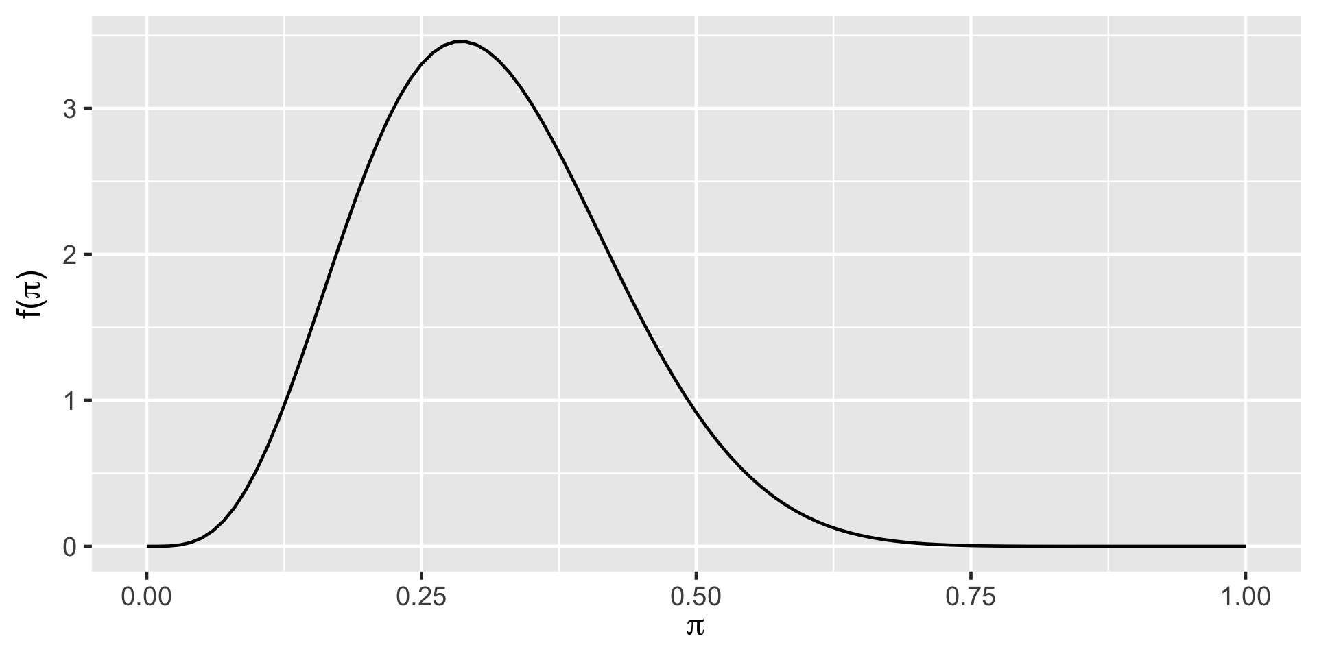
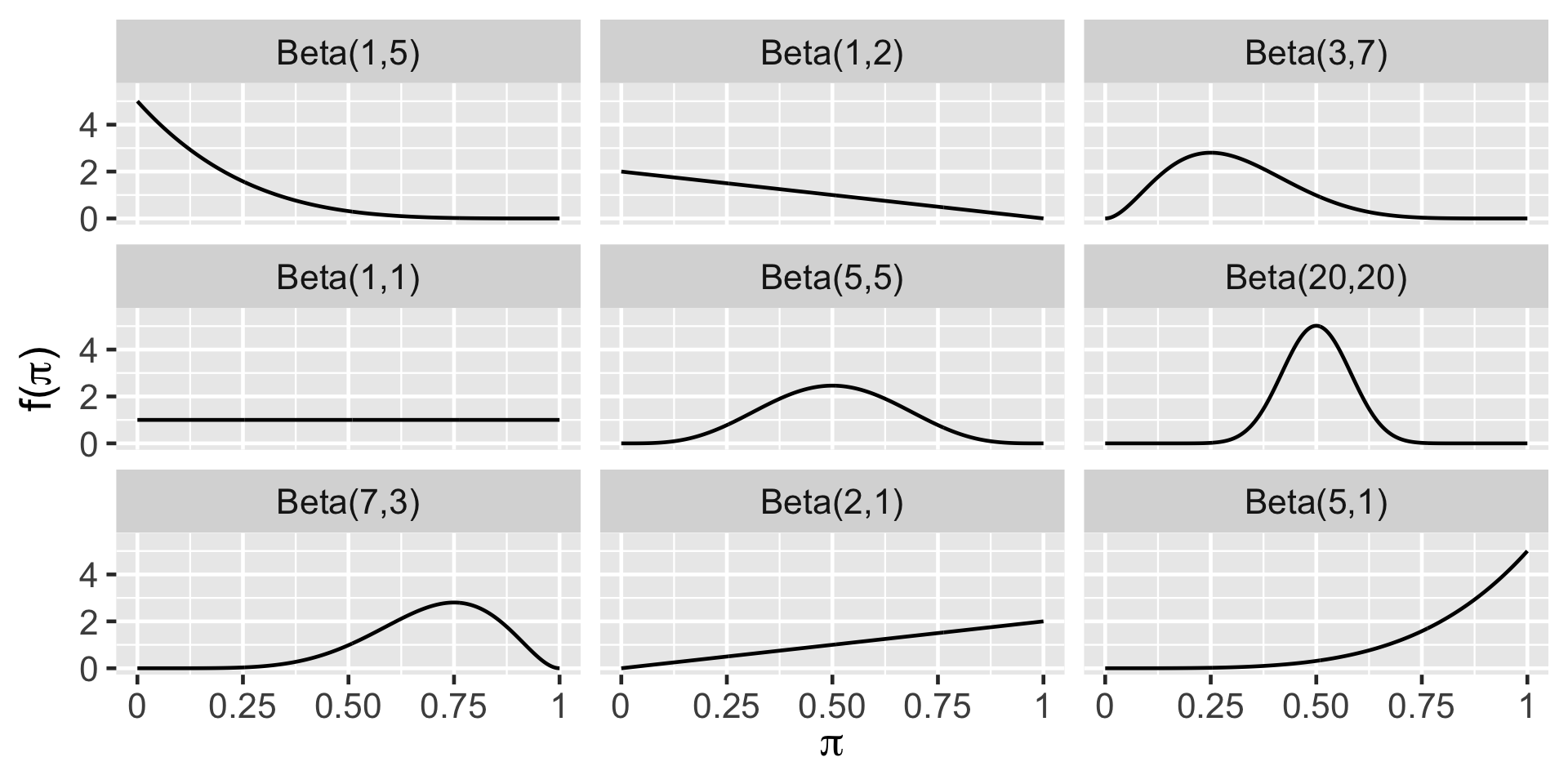
Plotting Beta Prior
The Optimist
plot_beta_binomial(14, 1, y = 9, n = 20)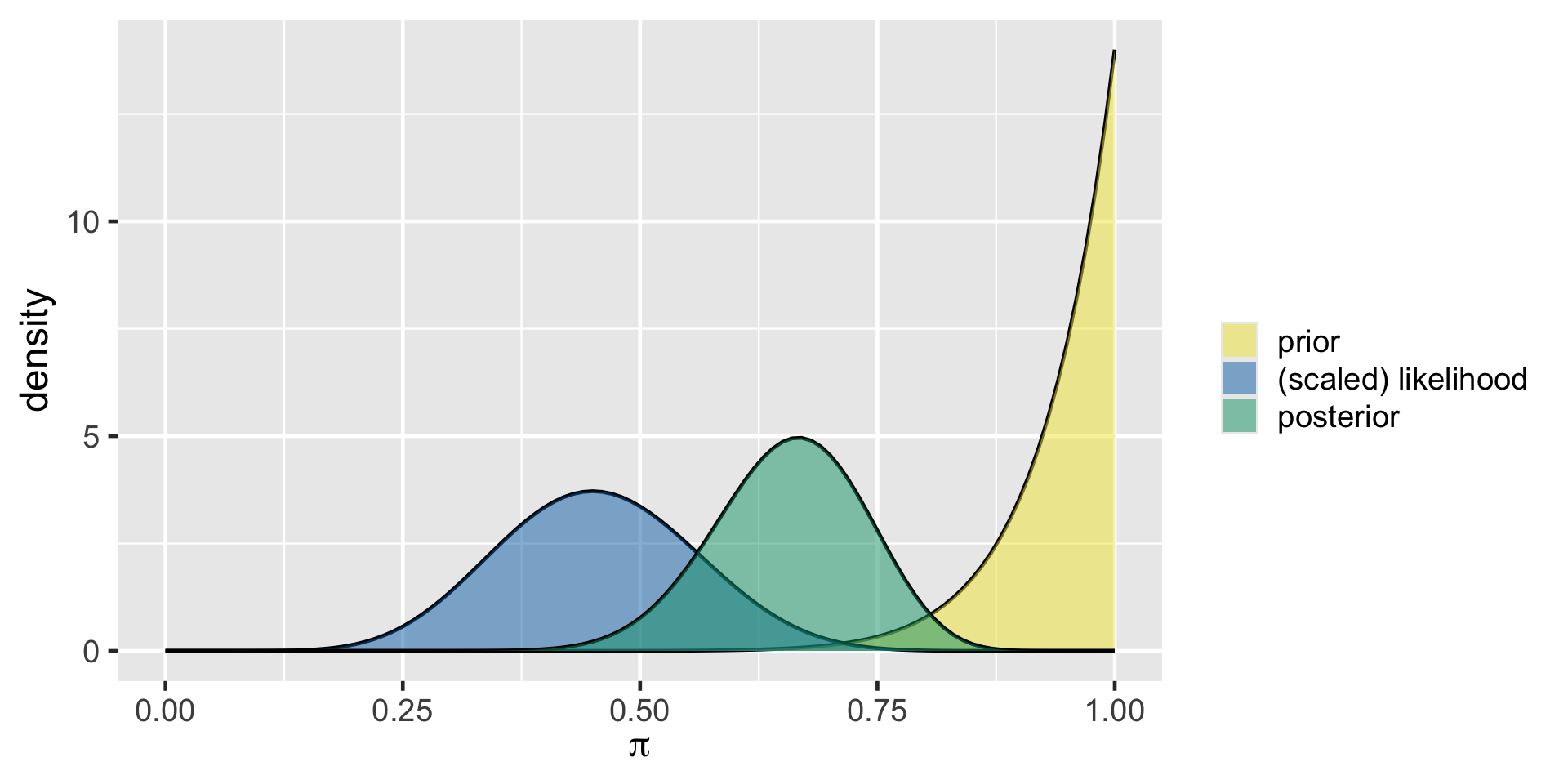
The Clueless
plot_beta_binomial(1, 1, y = 9, n = 20)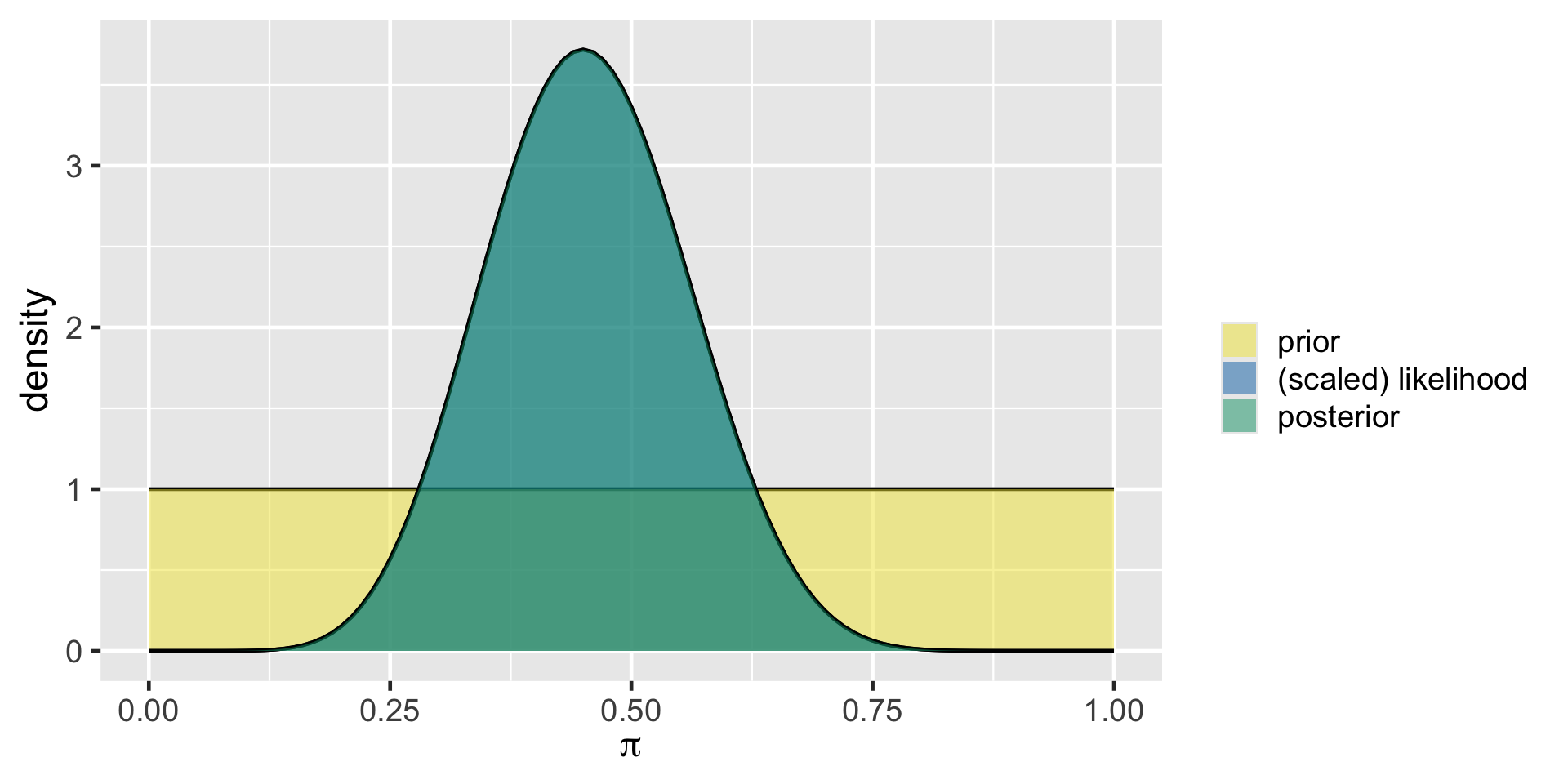
The Feminist
plot_beta_binomial(5, 11, y = 9, n = 20)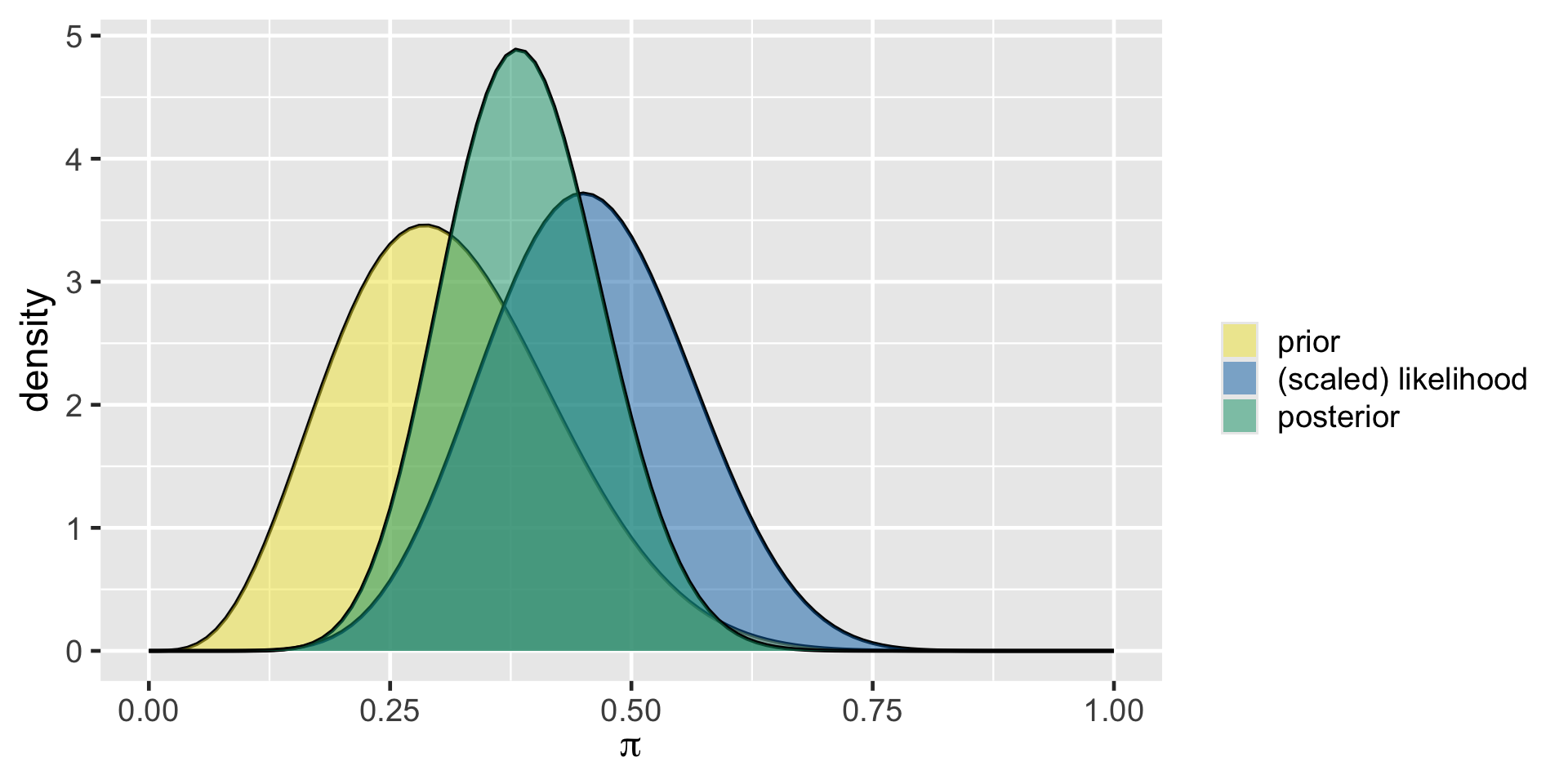
Comparison
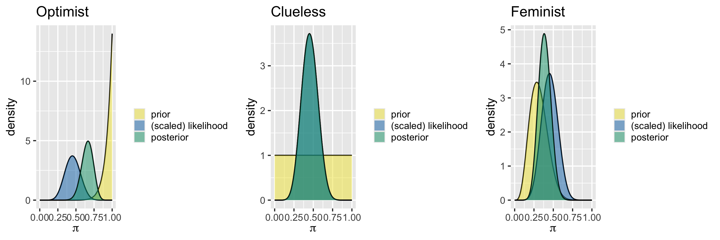
Balancing Act of Bayesian Analysis
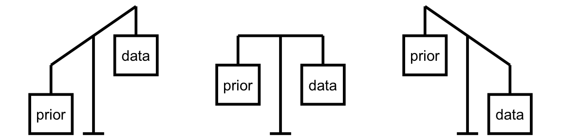
In Bayesian methodology, the prior model and the data both contribute to our posterior model.
Morteza’s analysis
plot_beta_binomial(14, 1, y = 6, n = 13)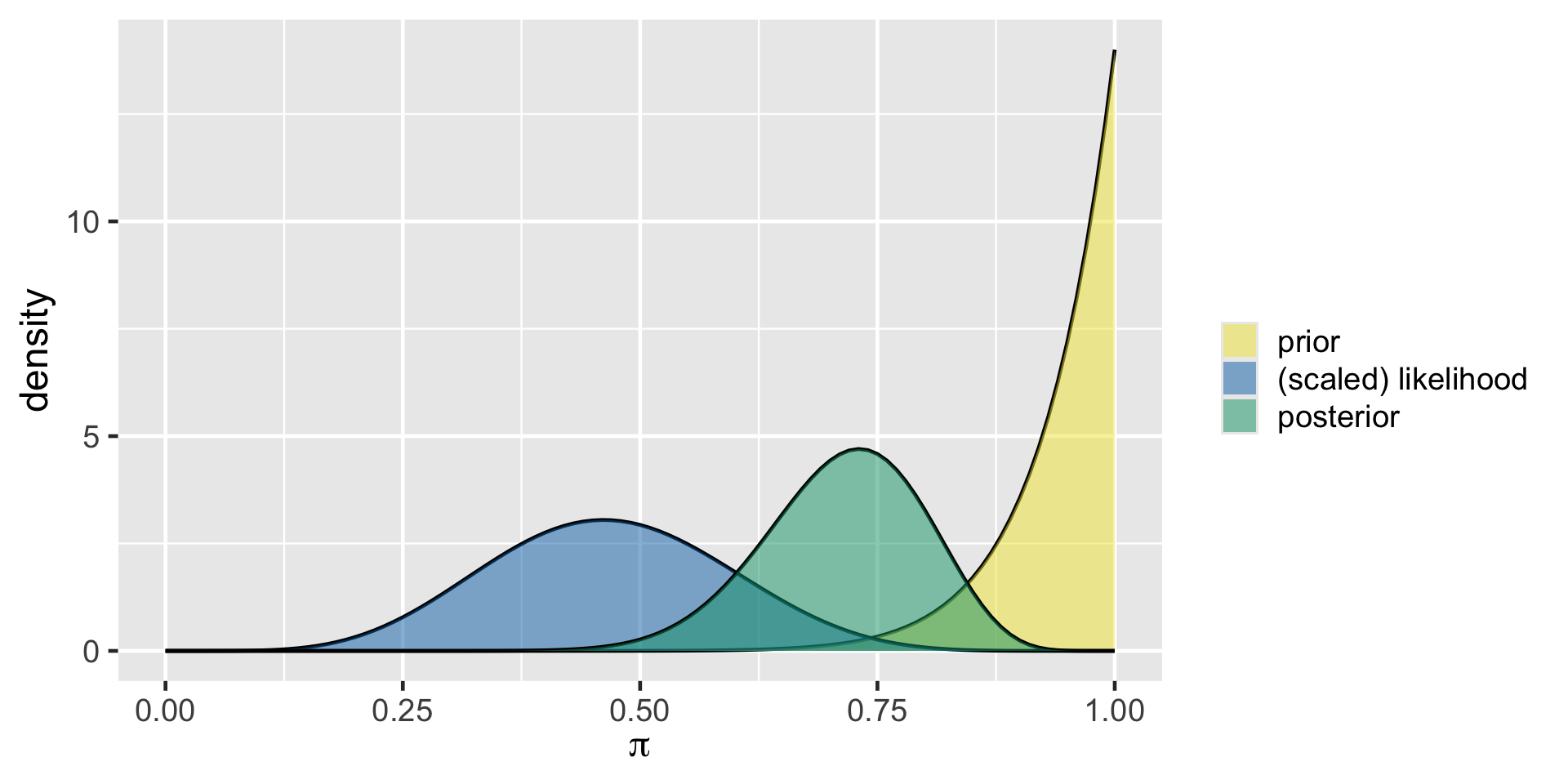
Nadide’s analysis
plot_beta_binomial(14, 1, y = 29, n = 63)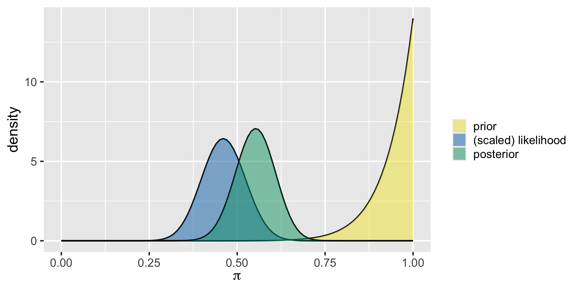
Ursula’s analysis
plot_beta_binomial(14, 1, y = 46, n = 99)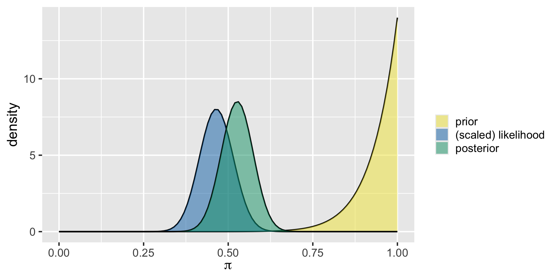
Summary
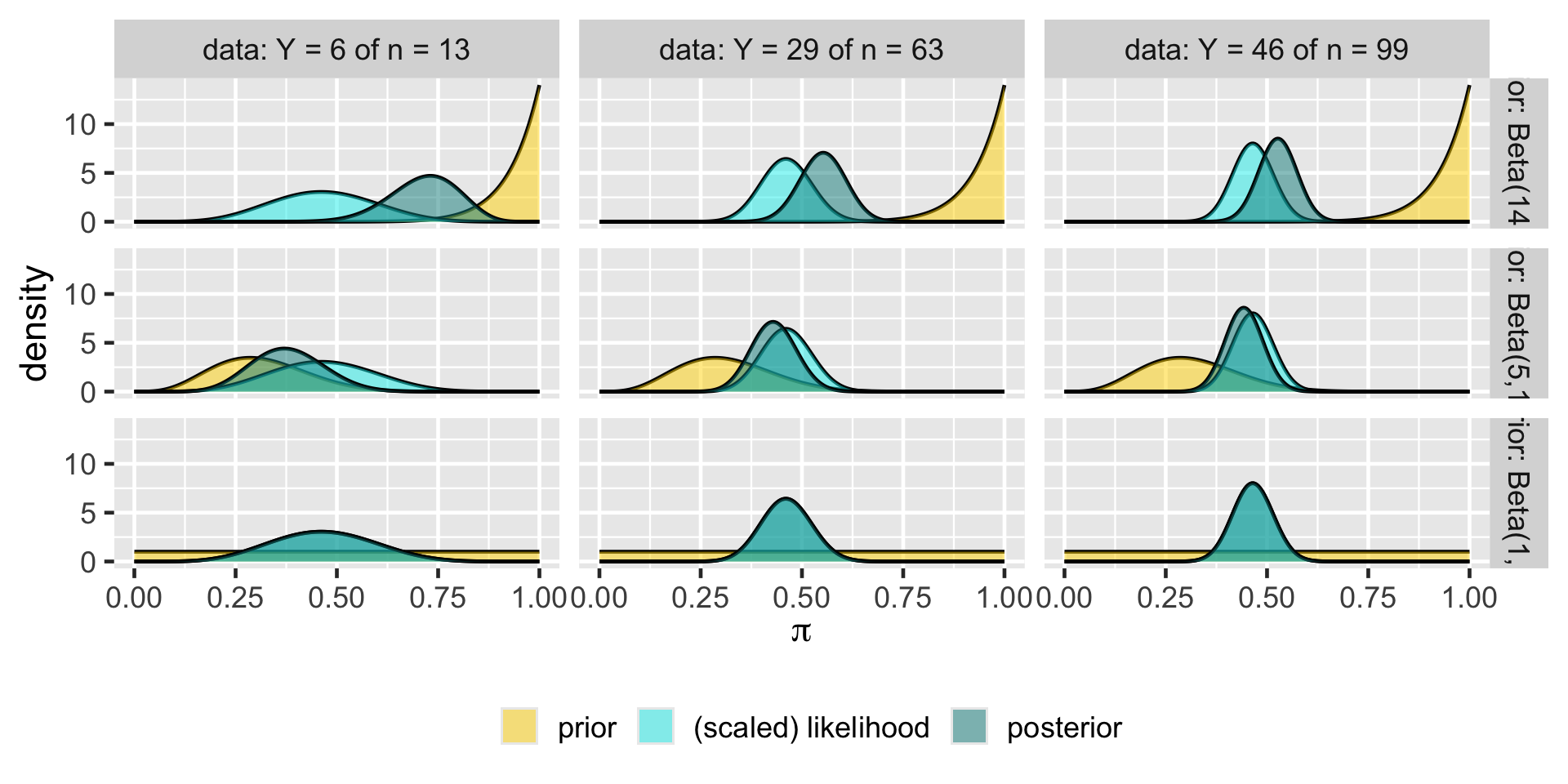
priors: Beta(14,1), Beta(5,11), Beta(1,1)