library(bayesrules)
library(tidyverse)Introduction to Bayesian Inference
Credible Intervals and Hypothesis Testing
Dr. Mine Dogucu
Packages
Examples from this lecture are mainly taken from the Bayes Rules! book and the new functions are from the bayesrules package.
Recall
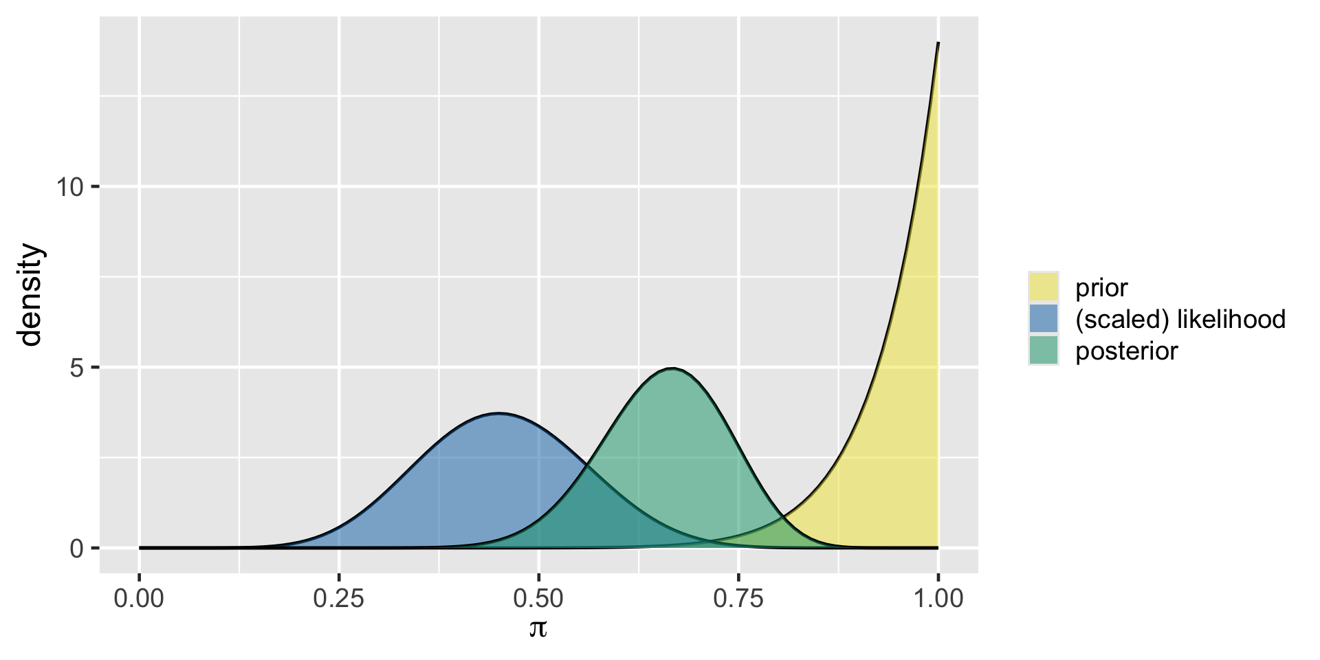
Last lecture the optimist had the following models.
      model alpha beta      mean      mode         var         sd
1     prior    14    1 0.9333333 1.0000000 0.003888889 0.06236096
2 posterior    23   12 0.6571429 0.6666667 0.006258503 0.07911070
Prior model: \(\pi \sim \text{Beta}(14, 1)\)
We can read this as the variable \(\pi\) follows a Beta model with parameters 14 and 1.
Posterior model: \(\pi|Y \sim \text{Beta}(23, 12)\)
We can read this as \(\pi\) given \(Y\) (i.e., the data) follows a Beta model with parameters 23 and 12.
Recall
Credible Intervals
Understanding Change of Beliefs
We are often interested in how our ideas change from prior to posterior.
One measure that can capture this change is the credible interval.
Prior credible interval
According to optimist’s prior model the probability that \(\pi\) is between 0.7683642 and 0.9981932 is 95%.
95% prior credible interval
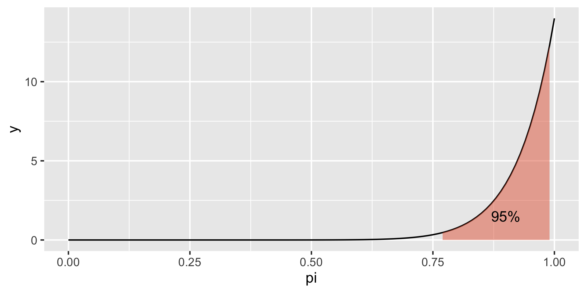
95% prior credible interval
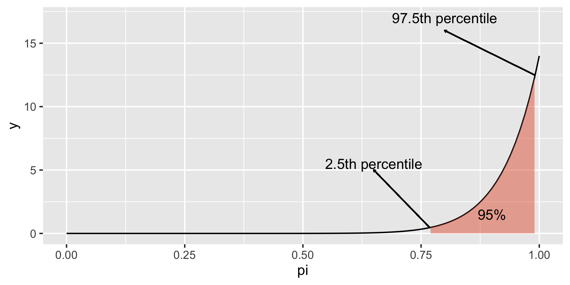
Prior Credible Interval
We can utilize the qbeta() function to calculate the middle 95% prior credible interval.
For a given quantile (probability) the qbeta() function returns the corresponding \(\pi\) value.
We are essentially calculating the 2.5th and 97.5th percentiles.
Posterior credible interval
After having observed the data, optimist’s posterior model indicates that with 95% probability \(\pi\) is between 0.4947347 and 0.8025414.
Hypothesis Testing
Recall feminist’s data analysis
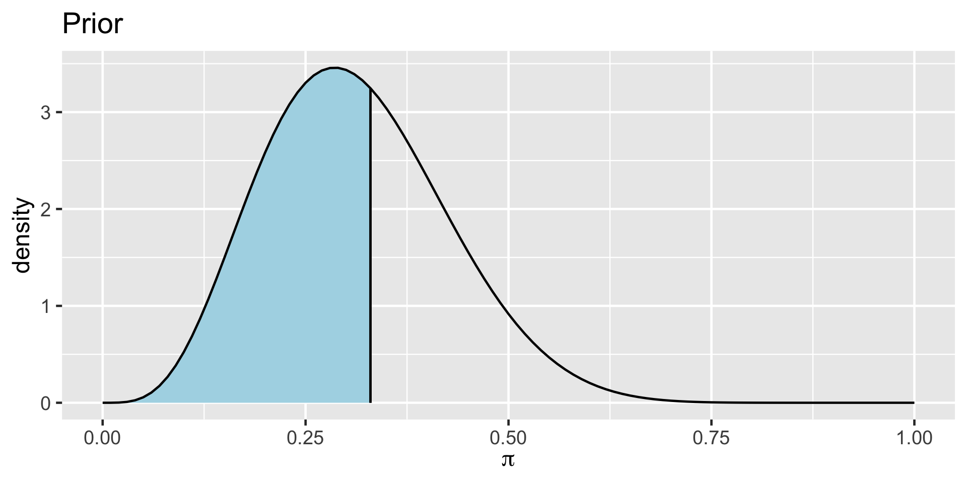
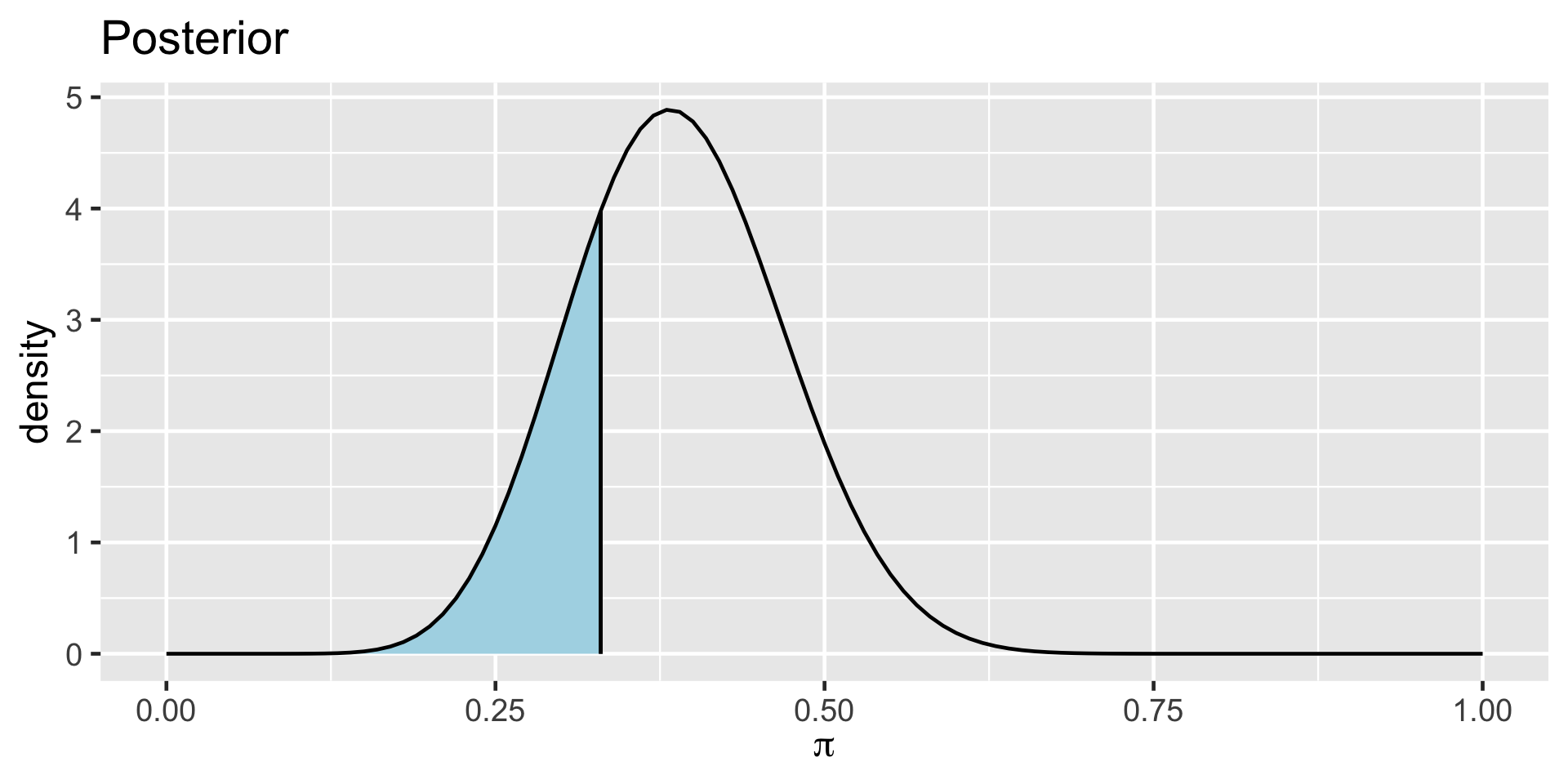
      model alpha beta      mean      mode        var         sd
1     prior     5   11 0.3125000 0.2857143 0.01263787 0.11241827
2 posterior    14   22 0.3888889 0.3823529 0.00642309 0.08014418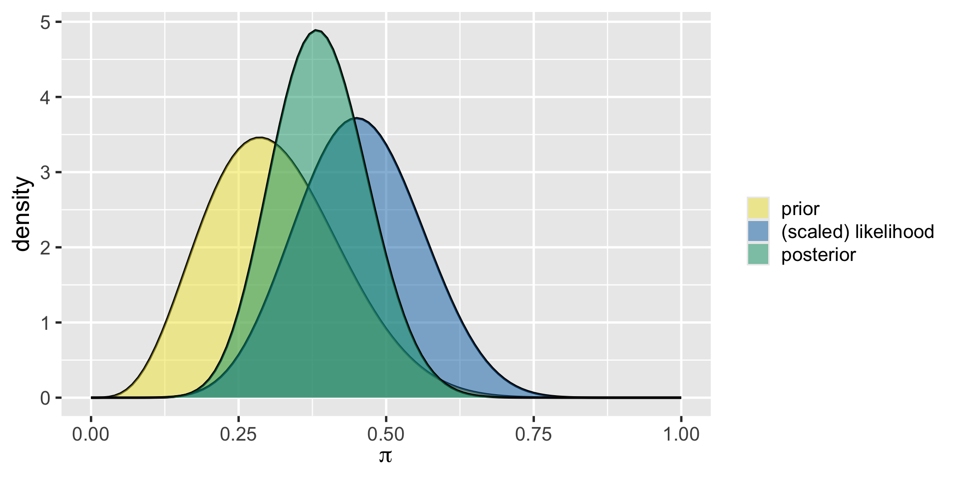
Scenario
Let’s assume that the general public assumes that more than one-third of the movies pass the Bechdel test. In other words, they believe \(\pi \geq 0.33\).
While working on his prior model, the feminist was unsure of this and wanted to put this claim to test during his data analysis.
Setting hypotheses
\(H_0: \pi \geq 0.33\)
\(H_A: \pi < 0.33\)
The null hypothesis (\(H_0\)) represents the status quo and the alternative hypothesis, (\(H_a\)), is feminist’s claim that he’d like to test.
Prior Probability
What is the prior probability that \(\pi\) is less than 0.33 ? In other words \(P(\pi < 0.33) = ?\)
Posterior Probability
What is the posterior probability that \(\pi\) is less than 0.33 after having observed the data? In other words \(P(\pi |Y < 0.33) = ?\)
Prior Model
Posterior Model
Prior odds
\[P(\pi<0.33)\]
Posterior odds
\[P(\pi | Y <0.33)\]
Bayes Factor
The Bayes Factor (BF) compares the posterior odds to the prior odds, hence provides insight into just how much the feminist’s understanding about movies passing the Bechdel test evolved upon observing the sample data:
\[\text{Bayes Factor} = \frac{\text{Posterior odds }}{\text{Prior odds }}\]
Bayes Factor
In a hypothesis test of two competing hypotheses, \(H_a\) vs \(H_0\), the Bayes Factor is an odds ratio for \(H_a\):
\[\text{Bayes Factor} = \frac{\text{Posterior odds}}{\text{Prior odds}} = \frac{P(H_a | Y) / P(H_0 | Y)}{P(H_a) / P(H_0)} \; .\]
Interpretation of BF
As a ratio, it’s meaningful to compare the Bayes Factor (BF) to 1. To this end, consider three possible scenarios:
- BF = 1: The plausibility of \(H_a\) didn’t change in light of the observed data.
- BF > 1: The plausibility of \(H_a\) increased in light of the observed data. Thus the greater the Bayes Factor, the more convincing the evidence for \(H_a\).
- BF < 1: The plausibility of \(H_a\) decreased in light of the observed data.