Multiple Linear Regression, Transformations, and Model Evaluation

Dr. Mine Dogucu

Data `babies` in `openintro` package

Rows: 1,236
Columns: 8
$ case      <int> 1, 2, 3, 4, 5, 6, 7, 8, 9, 10, 11, 12, 13, 14, 15, 16, 17, 1…
$ bwt       <int> 120, 113, 128, 123, 108, 136, 138, 132, 120, 143, 140, 144, …
$ gestation <int> 284, 282, 279, NA, 282, 286, 244, 245, 289, 299, 351, 282, 2…
$ parity    <int> 0, 0, 0, 0, 0, 0, 0, 0, 0, 0, 0, 0, 0, 0, 0, 0, 0, 0, 0, 0, …
$ age       <int> 27, 33, 28, 36, 23, 25, 33, 23, 25, 30, 27, 32, 23, 36, 30, …
$ height    <int> 62, 64, 64, 69, 67, 62, 62, 65, 62, 66, 68, 64, 63, 61, 63, …
$ weight    <int> 100, 135, 115, 190, 125, 93, 178, 140, 125, 136, 120, 124, 1…
$ smoke     <int> 0, 0, 1, 0, 1, 0, 0, 0, 0, 1, 0, 1, 1, 1, 0, 0, 1, 1, 0, 1, …

Variables

y	Response	Birth weight	Numeric
\(x_1\)	Explanatory	Gestation	Numeric
\(x_2\)	Explanatory	Smoke	Categorical

Notation

\(y_i = \beta_0 +\beta_1x_{1i} + \beta_2x_{2i} + \epsilon_i\)

\(\beta_0\) is intercept
\(\beta_1\) is the slope for gestation
\(\beta_2\) is the slope for smoke
\(\epsilon_i\) is error/residual
\(i = 1, 2, ...n\) identifier for each point

Model with gestation and smoke as predictos

model_gs <- lm(bwt ~ gestation + smoke, data = babies)
tidy(model_gs)

# A tibble: 3 × 5
  term        estimate std.error statistic  p.value
  <chr>          <dbl>     <dbl>     <dbl>    <dbl>
1 (Intercept)   -0.932    8.15      -0.114 9.09e- 1
2 gestation      0.443    0.0290    15.3   3.16e-48
3 smoke         -8.09     0.953     -8.49  5.96e-17

Expected birth weight

Expected birth weight for a baby who had 280 days of gestation with a smoker mother

\(\hat {\text{bwt}_i} = b_0 + b_1 \text{ gestation}_i + b_2 \text{ smoke}_i\)

\(\hat {\text{bwt}_i} = -0.932 + (0.443 \times 280) + (-8.09 \times 1)\)

Adding predictions

babies |> 
  modelr::add_predictions(model_gs) |> 
  select(bwt, gestation, smoke, pred)

# A tibble: 1,236 × 4
     bwt gestation smoke  pred
   <int>     <int> <int> <dbl>
 1   120       284     0  125.
 2   113       282     0  124.
 3   128       279     1  115.
 4   123        NA     0   NA 
 5   108       282     1  116.
 6   136       286     0  126.
 7   138       244     0  107.
 8   132       245     0  108.
 9   120       289     0  127.
10   143       299     1  123.
# ℹ 1,226 more rows

Adding residuals

babies |> 
  modelr::add_predictions(model_gs) |> 
  modelr::add_residuals(model_gs) |> 
  select(bwt, gestation, smoke, pred, resid)

# A tibble: 1,236 × 5
     bwt gestation smoke  pred  resid
   <int>     <int> <int> <dbl>  <dbl>
 1   120       284     0  125.  -4.84
 2   113       282     0  124. -11.0 
 3   128       279     1  115.  13.5 
 4   123        NA     0   NA   NA   
 5   108       282     1  116.  -7.87
 6   136       286     0  126.  10.3 
 7   138       244     0  107.  30.9 
 8   132       245     0  108.  24.4 
 9   120       289     0  127.  -7.05
10   143       299     1  123.  19.6 
# ℹ 1,226 more rows

Transformations

Data

library(AmesHousing)
ames_raw <- janitor::clean_names(ames_raw)
glimpse(ames_raw)

Rows: 2,930
Columns: 82
$ order           <int> 1, 2, 3, 4, 5, 6, 7, 8, 9, 10, 11, 12, 13, 14, 15, 16,…
$ pid             <chr> "0526301100", "0526350040", "0526351010", "0526353030"…
$ ms_sub_class    <chr> "020", "020", "020", "020", "060", "060", "120", "120"…
$ ms_zoning       <chr> "RL", "RH", "RL", "RL", "RL", "RL", "RL", "RL", "RL", …
$ lot_frontage    <int> 141, 80, 81, 93, 74, 78, 41, 43, 39, 60, 75, NA, 63, 8…
$ lot_area        <int> 31770, 11622, 14267, 11160, 13830, 9978, 4920, 5005, 5…
$ street          <chr> "Pave", "Pave", "Pave", "Pave", "Pave", "Pave", "Pave"…
$ alley           <chr> NA, NA, NA, NA, NA, NA, NA, NA, NA, NA, NA, NA, NA, NA…
$ lot_shape       <chr> "IR1", "Reg", "IR1", "Reg", "IR1", "IR1", "Reg", "IR1"…
$ land_contour    <chr> "Lvl", "Lvl", "Lvl", "Lvl", "Lvl", "Lvl", "Lvl", "HLS"…
$ utilities       <chr> "AllPub", "AllPub", "AllPub", "AllPub", "AllPub", "All…
$ lot_config      <chr> "Corner", "Inside", "Corner", "Corner", "Inside", "Ins…
$ land_slope      <chr> "Gtl", "Gtl", "Gtl", "Gtl", "Gtl", "Gtl", "Gtl", "Gtl"…
$ neighborhood    <chr> "NAmes", "NAmes", "NAmes", "NAmes", "Gilbert", "Gilber…
$ condition_1     <chr> "Norm", "Feedr", "Norm", "Norm", "Norm", "Norm", "Norm…
$ condition_2     <chr> "Norm", "Norm", "Norm", "Norm", "Norm", "Norm", "Norm"…
$ bldg_type       <chr> "1Fam", "1Fam", "1Fam", "1Fam", "1Fam", "1Fam", "Twnhs…
$ house_style     <chr> "1Story", "1Story", "1Story", "1Story", "2Story", "2St…
$ overall_qual    <int> 6, 5, 6, 7, 5, 6, 8, 8, 8, 7, 6, 6, 6, 7, 8, 8, 8, 9, …
$ overall_cond    <int> 5, 6, 6, 5, 5, 6, 5, 5, 5, 5, 5, 7, 5, 5, 5, 5, 7, 2, …
$ year_built      <int> 1960, 1961, 1958, 1968, 1997, 1998, 2001, 1992, 1995, …
$ year_remod_add  <int> 1960, 1961, 1958, 1968, 1998, 1998, 2001, 1992, 1996, …
$ roof_style      <chr> "Hip", "Gable", "Hip", "Hip", "Gable", "Gable", "Gable…
$ roof_matl       <chr> "CompShg", "CompShg", "CompShg", "CompShg", "CompShg",…
$ exterior_1st    <chr> "BrkFace", "VinylSd", "Wd Sdng", "BrkFace", "VinylSd",…
$ exterior_2nd    <chr> "Plywood", "VinylSd", "Wd Sdng", "BrkFace", "VinylSd",…
$ mas_vnr_type    <chr> "Stone", "None", "BrkFace", "None", "None", "BrkFace",…
$ mas_vnr_area    <int> 112, 0, 108, 0, 0, 20, 0, 0, 0, 0, 0, 0, 0, 0, 0, 603,…
$ exter_qual      <chr> "TA", "TA", "TA", "Gd", "TA", "TA", "Gd", "Gd", "Gd", …
$ exter_cond      <chr> "TA", "TA", "TA", "TA", "TA", "TA", "TA", "TA", "TA", …
$ foundation      <chr> "CBlock", "CBlock", "CBlock", "CBlock", "PConc", "PCon…
$ bsmt_qual       <chr> "TA", "TA", "TA", "TA", "Gd", "TA", "Gd", "Gd", "Gd", …
$ bsmt_cond       <chr> "Gd", "TA", "TA", "TA", "TA", "TA", "TA", "TA", "TA", …
$ bsmt_exposure   <chr> "Gd", "No", "No", "No", "No", "No", "Mn", "No", "No", …
$ bsmt_fin_type_1 <chr> "BLQ", "Rec", "ALQ", "ALQ", "GLQ", "GLQ", "GLQ", "ALQ"…
$ bsmt_fin_sf_1   <int> 639, 468, 923, 1065, 791, 602, 616, 263, 1180, 0, 0, 9…
$ bsmt_fin_type_2 <chr> "Unf", "LwQ", "Unf", "Unf", "Unf", "Unf", "Unf", "Unf"…
$ bsmt_fin_sf_2   <int> 0, 144, 0, 0, 0, 0, 0, 0, 0, 0, 0, 0, 0, 0, 1120, 0, 0…
$ bsmt_unf_sf     <int> 441, 270, 406, 1045, 137, 324, 722, 1017, 415, 994, 76…
$ total_bsmt_sf   <int> 1080, 882, 1329, 2110, 928, 926, 1338, 1280, 1595, 994…
$ heating         <chr> "GasA", "GasA", "GasA", "GasA", "GasA", "GasA", "GasA"…
$ heating_qc      <chr> "Fa", "TA", "TA", "Ex", "Gd", "Ex", "Ex", "Ex", "Ex", …
$ central_air     <chr> "Y", "Y", "Y", "Y", "Y", "Y", "Y", "Y", "Y", "Y", "Y",…
$ electrical      <chr> "SBrkr", "SBrkr", "SBrkr", "SBrkr", "SBrkr", "SBrkr", …
$ x1st_flr_sf     <int> 1656, 896, 1329, 2110, 928, 926, 1338, 1280, 1616, 102…
$ x2nd_flr_sf     <int> 0, 0, 0, 0, 701, 678, 0, 0, 0, 776, 892, 0, 676, 0, 0,…
$ low_qual_fin_sf <int> 0, 0, 0, 0, 0, 0, 0, 0, 0, 0, 0, 0, 0, 0, 0, 0, 0, 0, …
$ gr_liv_area     <int> 1656, 896, 1329, 2110, 1629, 1604, 1338, 1280, 1616, 1…
$ bsmt_full_bath  <int> 1, 0, 0, 1, 0, 0, 1, 0, 1, 0, 0, 1, 0, 1, 1, 1, 0, 1, …
$ bsmt_half_bath  <int> 0, 0, 0, 0, 0, 0, 0, 0, 0, 0, 0, 0, 0, 0, 0, 0, 0, 0, …
$ full_bath       <int> 1, 1, 1, 2, 2, 2, 2, 2, 2, 2, 2, 2, 2, 1, 1, 3, 2, 1, …
$ half_bath       <int> 0, 0, 1, 1, 1, 1, 0, 0, 0, 1, 1, 0, 1, 1, 1, 1, 0, 1, …
$ bedroom_abv_gr  <int> 3, 2, 3, 3, 3, 3, 2, 2, 2, 3, 3, 3, 3, 2, 1, 4, 4, 1, …
$ kitchen_abv_gr  <int> 1, 1, 1, 1, 1, 1, 1, 1, 1, 1, 1, 1, 1, 1, 1, 1, 1, 1, …
$ kitchen_qual    <chr> "TA", "TA", "Gd", "Ex", "TA", "Gd", "Gd", "Gd", "Gd", …
$ tot_rms_abv_grd <int> 7, 5, 6, 8, 6, 7, 6, 5, 5, 7, 7, 6, 7, 5, 4, 12, 8, 8,…
$ functional      <chr> "Typ", "Typ", "Typ", "Typ", "Typ", "Typ", "Typ", "Typ"…
$ fireplaces      <int> 2, 0, 0, 2, 1, 1, 0, 0, 1, 1, 1, 0, 1, 1, 0, 1, 0, 1, …
$ fireplace_qu    <chr> "Gd", NA, NA, "TA", "TA", "Gd", NA, NA, "TA", "TA", "T…
$ garage_type     <chr> "Attchd", "Attchd", "Attchd", "Attchd", "Attchd", "Att…
$ garage_yr_blt   <int> 1960, 1961, 1958, 1968, 1997, 1998, 2001, 1992, 1995, …
$ garage_finish   <chr> "Fin", "Unf", "Unf", "Fin", "Fin", "Fin", "Fin", "RFn"…
$ garage_cars     <int> 2, 1, 1, 2, 2, 2, 2, 2, 2, 2, 2, 2, 2, 2, 2, 3, 2, 3, …
$ garage_area     <int> 528, 730, 312, 522, 482, 470, 582, 506, 608, 442, 440,…
$ garage_qual     <chr> "TA", "TA", "TA", "TA", "TA", "TA", "TA", "TA", "TA", …
$ garage_cond     <chr> "TA", "TA", "TA", "TA", "TA", "TA", "TA", "TA", "TA", …
$ paved_drive     <chr> "P", "Y", "Y", "Y", "Y", "Y", "Y", "Y", "Y", "Y", "Y",…
$ wood_deck_sf    <int> 210, 140, 393, 0, 212, 360, 0, 0, 237, 140, 157, 483, …
$ open_porch_sf   <int> 62, 0, 36, 0, 34, 36, 0, 82, 152, 60, 84, 21, 75, 0, 5…
$ enclosed_porch  <int> 0, 0, 0, 0, 0, 0, 170, 0, 0, 0, 0, 0, 0, 0, 0, 0, 0, 0…
$ x3ssn_porch     <int> 0, 0, 0, 0, 0, 0, 0, 0, 0, 0, 0, 0, 0, 0, 0, 0, 0, 0, …
$ screen_porch    <int> 0, 120, 0, 0, 0, 0, 0, 144, 0, 0, 0, 0, 0, 0, 140, 210…
$ pool_area       <int> 0, 0, 0, 0, 0, 0, 0, 0, 0, 0, 0, 0, 0, 0, 0, 0, 0, 0, …
$ pool_qc         <chr> NA, NA, NA, NA, NA, NA, NA, NA, NA, NA, NA, NA, NA, NA…
$ fence           <chr> NA, "MnPrv", NA, NA, "MnPrv", NA, NA, NA, NA, NA, NA, …
$ misc_feature    <chr> NA, NA, "Gar2", NA, NA, NA, NA, NA, NA, NA, NA, "Shed"…
$ misc_val        <int> 0, 0, 12500, 0, 0, 0, 0, 0, 0, 0, 0, 500, 0, 0, 0, 0, …
$ mo_sold         <int> 5, 6, 6, 4, 3, 6, 4, 1, 3, 6, 4, 3, 5, 2, 6, 6, 6, 6, …
$ yr_sold         <int> 2010, 2010, 2010, 2010, 2010, 2010, 2010, 2010, 2010, …
$ sale_type       <chr> "WD ", "WD ", "WD ", "WD ", "WD ", "WD ", "WD ", "WD "…
$ sale_condition  <chr> "Normal", "Normal", "Normal", "Normal", "Normal", "Nor…
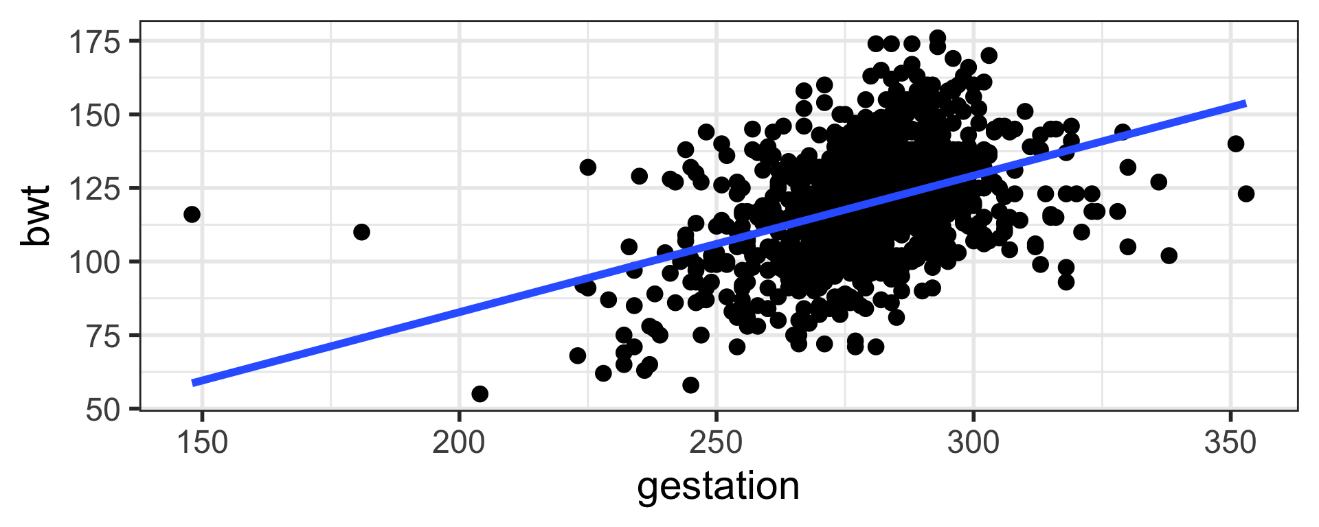
$ sale_price      <int> 215000, 105000, 172000, 244000, 189900, 195500, 213500…

Visual inspection

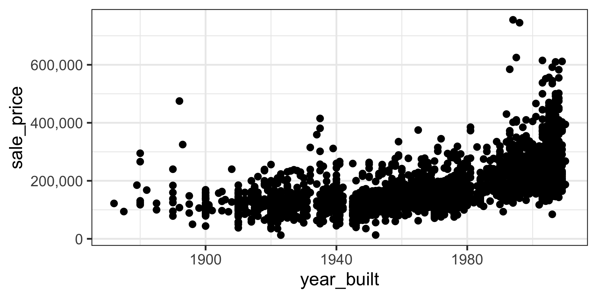
A scatter plot displays "sale_price" on the y-axis, ranging from 0 to over 600,000, against "year_built" on the x-axis, ranging from approximately 1860 to 2000. Numerous black data points illustrate a general positive trend, with sale prices tending to increase for more recently built properties. The density of data points is higher for houses built after 1980, and the variability in sale prices also visibly increases for more recent build years, showing a clear pattern of unequal variance.

Visual inspection with transformation

A scatter plot displays the logarithm of sale price (log(sale_price)) on the y-axis, ranging from approximately 9.5 to 13, against year built on the x-axis, ranging from approximately 1860 to 2000. Numerous black data points illustrate a general positive trend, with log sale prices tending to increase for more recently built properties. The vertical spread of the data points appears relatively constant across the range of years built, suggesting a more consistent variability after the logarithmic transformation.

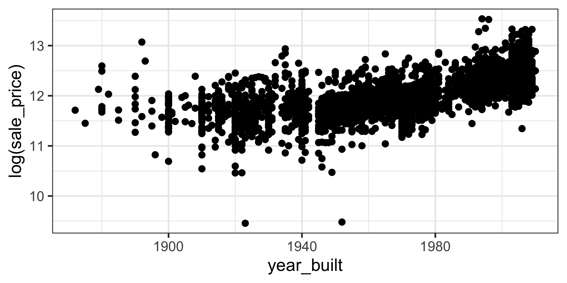
Note that log is natural log in R.

Model with log(y)

model_y <- lm(log(sale_price) ~ year_built, 
              data = ames_raw)
tidy(model_y)

# A tibble: 2 × 5
  term        estimate std.error statistic   p.value
  <chr>          <dbl>     <dbl>     <dbl>     <dbl>
1 (Intercept) -4.33     0.387        -11.2 1.73e- 28
2 year_built   0.00829  0.000196      42.3 4.45e-305

\({log(\hat y_i)} = b_0 + b_1x_{1i}\)

\({log(\hat y_i)} = -4.33 + 0.00829x_{1i}\)

Estimated y

Estimated sale price of a house built in 1980

\({log(\hat y_i)} = -4.33 + 0.00829 \times 1980\)

\(e^{log(\hat y_i)} = e^{-4.33 + 0.00829 \times 1980}\)

\(\hat y_i = e^{-4.33} \times e^ {0.00829 \times 1980} = 177052.2\)

For one-unit (year) increase in x, the y is multiplied by \(e^{b_1}\).

Note that \(e^x\) can be achieved by exp(x) in R.

Common Transformations

\(log(Y)\), \(log(X)\)
\(1/Y\), \(1/X\)
\(\sqrt{Y}, \sqrt{X})\)

Model Evaluation

glimpse(babies)

Rows: 1,236
Columns: 8
$ case      <int> 1, 2, 3, 4, 5, 6, 7, 8, 9, 10, 11, 12, 13, 14, 15, 16, 17, 1…
$ bwt       <int> 120, 113, 128, 123, 108, 136, 138, 132, 120, 143, 140, 144, …
$ gestation <int> 284, 282, 279, NA, 282, 286, 244, 245, 289, 299, 351, 282, 2…
$ parity    <int> 0, 0, 0, 0, 0, 0, 0, 0, 0, 0, 0, 0, 0, 0, 0, 0, 0, 0, 0, 0, …
$ age       <int> 27, 33, 28, 36, 23, 25, 33, 23, 25, 30, 27, 32, 23, 36, 30, …
$ height    <int> 62, 64, 64, 69, 67, 62, 62, 65, 62, 66, 68, 64, 63, 61, 63, …
$ weight    <int> 100, 135, 115, 190, 125, 93, 178, 140, 125, 136, 120, 124, 1…
$ smoke     <int> 0, 0, 1, 0, 1, 0, 0, 0, 0, 1, 0, 1, 1, 1, 0, 0, 1, 1, 0, 1, …

Back to `model_g`

model_g <- lm(bwt ~ gestation, data = babies)
tidy(model_g)

# A tibble: 2 × 5
  term        estimate std.error statistic  p.value
  <chr>          <dbl>     <dbl>     <dbl>    <dbl>
1 (Intercept)  -10.1      8.32       -1.21 2.27e- 1
2 gestation      0.464    0.0297     15.6  3.22e-50

Model evaluation criteria

glance(model_g)

# A tibble: 1 × 12
  r.squared adj.r.squared sigma statistic  p.value    df logLik    AIC    BIC
      <dbl>         <dbl> <dbl>     <dbl>    <dbl> <dbl>  <dbl>  <dbl>  <dbl>
1     0.166         0.166  16.7      244. 3.22e-50     1 -5175. 10356. 10371.
# ℹ 3 more variables: deviance <dbl>, df.residual <int>, nobs <int>

\(R^2\)

glance(model_g)$r.squared

[1] 0.1663449

16% of the variation in birth weight is explained by gestation. Higher values of R squared is preferred.

A scatter plot displays birth weight (bwt) on the y-axis, ranging from approximately 50 to 175, against gestational age (gestation) on the x-axis, ranging from approximately 150 to 350. There is a moderate positive relationship, indicating that birth weight generally increases with gestational age. The majority of data points form a dense cluster between 250-300 for gestation and 100-150 for bwt. Scattered points exist across the range, including some with lower birth weights for both very short and very long gestations. A prominent blue line is drawn through the data. This line slopes upwards, from approximately (150, 60) to (350, 155), visually summarizing the positive relationship. While the line indicates an average trend, the data points show considerable scatter around it, implying variability in birth weight for a given gestational age.

Model with gestation, smoke, and age

model_gsa <- lm(bwt ~ gestation + smoke + age, data = babies)

Adjusted R-Squared

glance(model_g)

# A tibble: 1 × 12
  r.squared adj.r.squared sigma statistic  p.value    df logLik    AIC    BIC
      <dbl>         <dbl> <dbl>     <dbl>    <dbl> <dbl>  <dbl>  <dbl>  <dbl>
1     0.166         0.166  16.7      244. 3.22e-50     1 -5175. 10356. 10371.
# ℹ 3 more variables: deviance <dbl>, df.residual <int>, nobs <int>

glance(model_gsa)

# A tibble: 1 × 12
  r.squared adj.r.squared sigma statistic  p.value    df logLik    AIC    BIC
      <dbl>         <dbl> <dbl>     <dbl>    <dbl> <dbl>  <dbl>  <dbl>  <dbl>
1     0.212         0.210  16.2      108. 3.45e-62     3 -5089. 10187. 10213.
# ℹ 3 more variables: deviance <dbl>, df.residual <int>, nobs <int>

When comparing models with multiple predictors we rely on Adjusted R-squared.

Add predictions and residuals

babies |> 
  add_predictions(model_g) |> 
  add_residuals(model_g) |> 
  select(bwt, pred, resid)

# A tibble: 1,236 × 3
     bwt  pred  resid
   <int> <dbl>  <dbl>
 1   120  122.  -1.79
 2   113  121.  -7.86
 3   128  119.   8.53
 4   123   NA   NA   
 5   108  121. -12.9 
 6   136  123.  13.3 
 7   138  103.  34.8 
 8   132  104.  28.3 
 9   120  124.  -4.11
10   143  129.  14.2 
# ℹ 1,226 more rows

Add predictions and residuals

babies |> 
  add_predictions(model_gsa) |> 
  add_residuals(model_gsa) |> 
  select(bwt, pred, resid)

# A tibble: 1,236 × 3
     bwt  pred  resid
   <int> <dbl>  <dbl>
 1   120  125.  -4.80
 2   113  125. -11.5 
 3   128  115.  13.3 
 4   123   NA   NA   
 5   108  115.  -7.47
 6   136  125.  10.5 
 7   138  108.  30.4 
 8   132  107.  25.0 
 9   120  127.  -6.81
10   143  124.  19.2 
# ℹ 1,226 more rows

Root Mean Square Error

\(RMSE = \sqrt{\frac{\Sigma_{i=1}^n(y_i-\hat y_i)^2}{n}}\)

RMSE comparison

modelr::rmse(model_gsa, babies)

[1] 16.1687

modelr::rmse(model_g, babies)

[1] 16.6512

Full Model

model_full <- lm(bwt ~ gestation + parity + age +
                   height + weight + smoke, 
                 data = babies)

modelr::rmse(model_full, babies)

[1] 15.78198

glance(model_full)$adj.r.squared

[1] 0.2541383

Can we keep adding all the variables and try to get an EXCELLENT model fit?

Overfitting

We are fitting the model to sample data.
Our goal is to understand the population data.
If we make our model too perfect for our sample data, the model may not perform as well with other sample data from the population.
In this case we would be overfitting the data.
We can use model validation techniques.

Splitting the Data (Train vs. Test)

set.seed(12345)
babies_split <- rsample::initial_split(babies) ## 75% to 25% split

babies_train <- rsample::training(babies_split)
dim(babies_train)

[1] 927   8

babies_test <- rsample::testing(babies_split)
dim(babies_test)

[1] 309   8

Fitting Models

model_gsa_train <- lm(bwt ~ gestation + smoke + age, data = babies_train)
model_gsa_test <- lm(bwt ~ gestation + smoke + age, data = babies_test)

In the training stage, once we confirm our “best” model then we test it with test data.

Comparison of model evaluation criteria for training and testing data

glance(model_gsa_train)

# A tibble: 1 × 12
  r.squared adj.r.squared sigma statistic  p.value    df logLik   AIC   BIC
      <dbl>         <dbl> <dbl>     <dbl>    <dbl> <dbl>  <dbl> <dbl> <dbl>
1     0.204         0.201  16.4      76.8 2.87e-44     3 -3815. 7641. 7665.
# ℹ 3 more variables: deviance <dbl>, df.residual <int>, nobs <int>

glance(model_gsa_test)

# A tibble: 1 × 12
  r.squared adj.r.squared sigma statistic  p.value    df logLik   AIC   BIC
      <dbl>         <dbl> <dbl>     <dbl>    <dbl> <dbl>  <dbl> <dbl> <dbl>
1     0.243         0.236  15.8      32.2 4.21e-18     3 -1272. 2553. 2572.
# ℹ 3 more variables: deviance <dbl>, df.residual <int>, nobs <int>

Comparison of model evaluation criteria for training and testing data

modelr::rmse(model_gsa_train, babies_train)

[1] 16.31741

modelr::rmse(model_gsa_test, babies_test)

[1] 15.64897

Multiple Linear Regression, Transformations, and Model Evaluation

Data babies in openintro package

Variables

Notation

Model with gestation and smoke as predictos

Expected birth weight

Adding predictions

Adding residuals

Transformations

Data

Visual inspection

Visual inspection with transformation

Model with log(y)

Estimated y

Common Transformations

Model Evaluation

Back to model_g

Model evaluation criteria

\(R^2\)

Model with gestation, smoke, and age

Adjusted R-Squared

Add predictions and residuals

Add predictions and residuals

Root Mean Square Error

RMSE comparison

Full Model

Overfitting

Splitting the Data (Train vs. Test)

Fitting Models

Comparison of model evaluation criteria for training and testing data

Comparison of model evaluation criteria for training and testing data

Data `babies` in `openintro` package

Back to `model_g`