Logistic Regression

Dr. Mine Dogucu

GitHub repos

No repo this week. Time for you to create your own repos under your own username. Make sure to set them to be private.

(Normal) Linear Regression Response Variables

Birth weight of Babies (55 - 176 ounces)
Sale Prices ($12789 - $755,000)
Number of Species (6 - 129 mammals)

Logistic Regression Response Variables

Will it rain tomorrow? (Yes/No)
Is email spam? (Yes/No)
Does the candidate receive a callback? (Yes/No)

When the response variable is binary a logistic regression model can be utilized.

Data source

Are Emily and Greg More Employable than Lakisha and Jamal? A Field Experiment on Labor Market Discrimination.

Data source

Researchers respond to help-wanted ads in Boston and Chicago newspapers with fictitious resumes.

They randomly assign White sounding names to half the resumes and African American sounding names to the other half.

They create high quality resumes (more experience, likely to have an email address etc.) and low quality resumes.
For each job ad they send four resumes (two high quality and two low quality.)

Data

resume <- resume |> 
  select(received_callback, race, years_experience, 
         job_city)

glimpse(resume)

Rows: 4,870
Columns: 4
$ received_callback <lgl> FALSE, FALSE, FALSE, FALSE, FALSE, FALSE, FALSE, FAL…
$ race              <chr> "white", "white", "black", "black", "white", "white"…
$ years_experience  <int> 6, 6, 6, 6, 22, 6, 5, 21, 3, 6, 8, 8, 4, 4, 5, 4, 5,…
$ job_city          <chr> "Chicago", "Chicago", "Chicago", "Chicago", "Chicago…

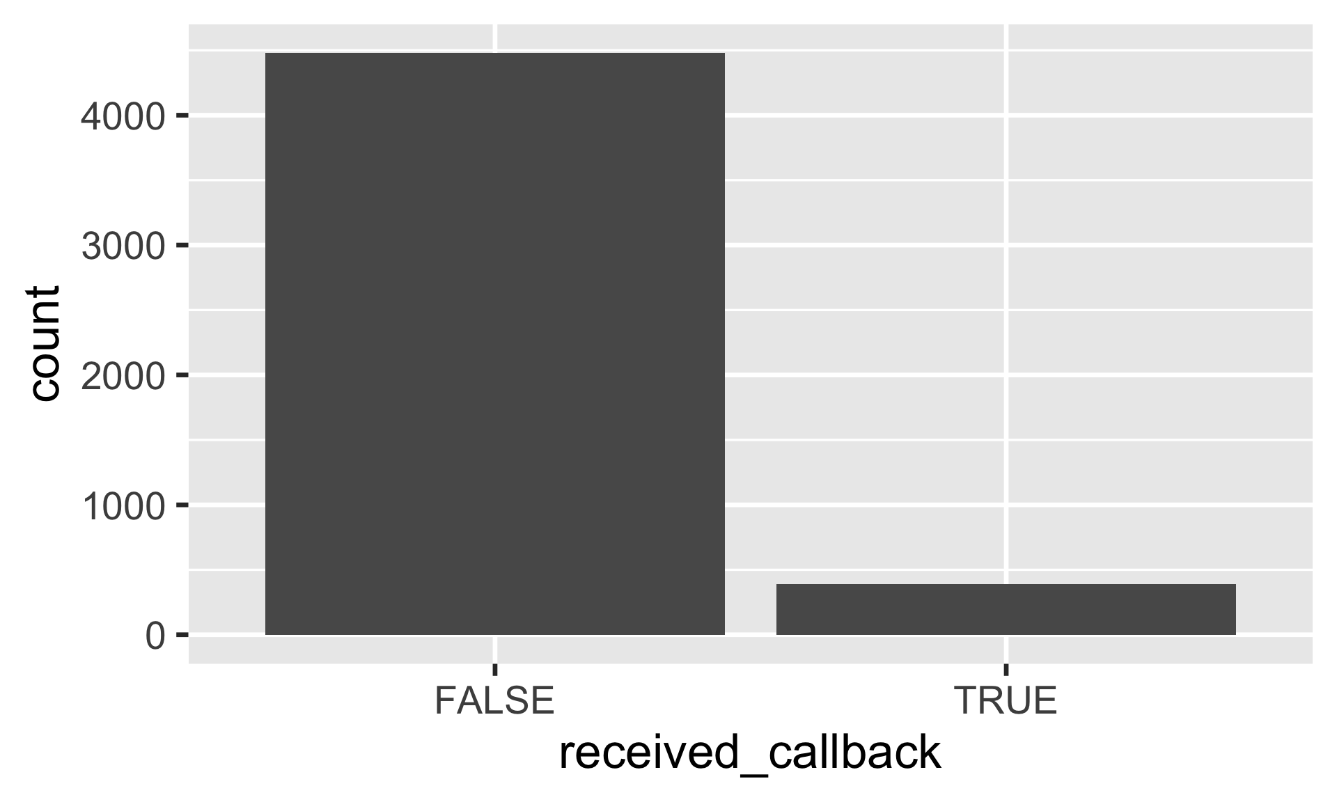
Response variable: `received_callback`

count(resume, received_callback) |> 
  mutate(prop = n / sum(n))

# A tibble: 2 × 3
  received_callback     n   prop
  <lgl>             <int>  <dbl>
1 FALSE              4478 0.920 
2 TRUE                392 0.0805

A bar chart titled "received_callback" displays the count of two categories on the y-axis, ranging from 0 to 4500. The x-axis shows two categories: "FALSE" and "TRUE". The bar for "FALSE" is significantly taller, reaching a count of approximately 4500. The bar for "TRUE" is much shorter, reaching a count of approximately 400. This indicates a large imbalance, with far fewer instances of "TRUE" compared to "FALSE".

Notation

$y_i$ = whether a (fictitious) job candidate receives a call back.

$\pi_i$ = probability that the $i$th job candidate will receive a call back.

$1-\pi_i$ = probability that the $i$th job candidate will not receive a call back.

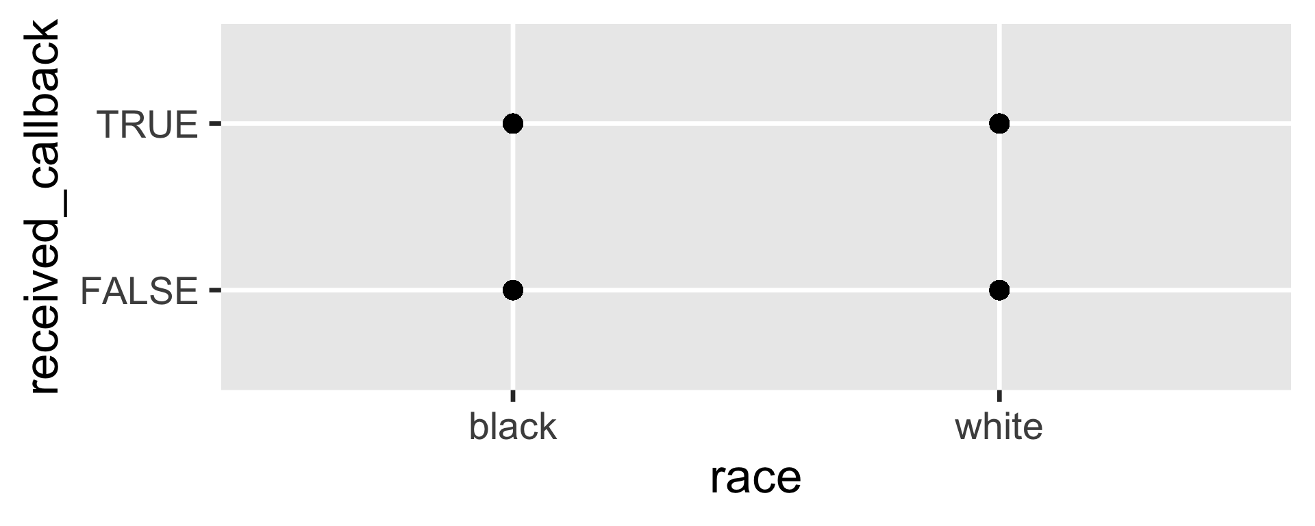
Where is the line?

ggplot(resume, aes(x = race, y = received_callback)) +
  geom_point()

A dot plot shows two categorical variables: "received_callback" on the y-axis (with categories FALSE and TRUE) and "race" on the x-axis (with categories black and white). A black dot is present for each combination of these categories: (black, FALSE), (black, TRUE), (white, FALSE), and (white, TRUE), indicating that data exists for all four combinations.

The Linear Model

We can model the probability of receiving a callback with a linear model.

$\text{transformation}(\pi_i) = \beta_0 + \beta_1x_{1i}+\beta_2x_{2i} +.... \beta_kx_{ki}$

$logit(\pi_i) = \beta_0 + \beta_1x_{1i}+\beta_2x_{2i} +.... \beta_kx_{ki}$

$logit(\pi_i) = log(\frac{\pi_i}{1-\pi_i})$

Note that log is natural log and not base 10. This is also the case for the log() function in R.

Probability, Odds, and Logit

Probability $\pi_i$ Probability of receiving a callback.

Odds $\frac{\pi_i}{1-\pi_i}$ Odds of receiving a callback.

Logit $log(\frac{\pi_i}{1-\pi_i})$ Logit of receiving a callback.

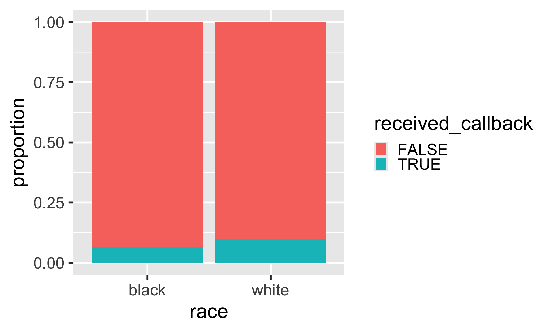
Proportion as outcome

A 100% stacked bar chart displays the proportion of "received_callback" (FALSE in red, TRUE in teal) for two "race" categories: "black" and "white". The y-axis represents proportion from 0 to 1.00. For both "black" and "white" categories, the vast majority of the bar is colored red, representing "FALSE", while a small teal segment at the bottom represents "TRUE". The teal "TRUE" segment for "white" appears slightly larger than for "black," indicating that a slightly higher proportion of "white" individuals received a callback compared to "black" individuals, though callbacks remain a small proportion for both groups.

When race is black (0)

resume |> 
  filter(race == "black") |> 
  count(received_callback) |> 
  mutate(prop = n / sum(n))

# A tibble: 2 × 3
  received_callback     n   prop
  <lgl>             <int>  <dbl>
1 FALSE              2278 0.936 
2 TRUE                157 0.0645

Note that R assigns 0 an 1 to levels of categorical variables in alphabetical order. In this case black (0) and white(1)

When race is black (0)

p_b <- resume |> 
  filter(race == "black") |> 
  count(received_callback) |> 
  mutate(prop = n / sum(n)) |> 
  filter(received_callback == TRUE) |> 
  select(prop) |> 
  pull()

Probability of receiving a callback when the candidate has a Black sounding name is 0.0644764.

When race is white (1)

p_w <- resume |> 
  filter(race == "white") |> 
  count(received_callback) |> 
  mutate(prop = n / sum(n)) |> 
  filter(received_callback == TRUE) |> 
  select(prop) |> 
  pull()

Probability of receiving a callback when the candidate has a white sounding name is 0.0965092.

Probability, Odds, and Logit

p_b

[1] 0.06447639

## Odds
odds_b <- p_b / (1 - p_b)
odds_b

[1] 0.06892011

## Logit
logit_b <- log(odds_b)
logit_b

[1] -2.674807

Probability, Odds, and Logit

p_b

[1] 0.06447639

## Odds
odds_b <- p_b / (1 - p_b)
odds_b

[1] 0.06892011

## Logit
logit_b <- log(odds_b)
logit_b

[1] -2.674807

p_w

[1] 0.09650924

## Odds
odds_w <- p_w / (1 - p_w)
odds_w

[1] 0.1068182

## Logit
logit_w <- log(odds_w)
logit_w

[1] -2.236627

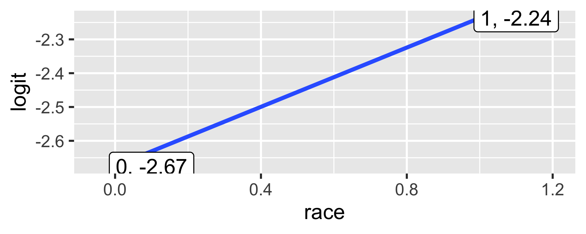
Estimates

A line plot displays "logit" on the y-axis, ranging from -2.6 to -2.2, against "race" on the x-axis, ranging from 0.0 to 1.2. A straight blue line connects two data points. The first point is at (0, -2.67), labeled as "0, -2.67". The second point is at (1, -2.24), labeled as "1, -2.24". The line shows a positive linear relationship, indicating that the logit value increases as "race" increases from 0 to 1.

This is THE LINE of the linear model. As x increases by 1 unit, the expected change in the logit of receiving call back is 0.4381802.

The slope of the line is:

logit_w - logit_b

[1] 0.4381802

The slope is the difference between logit for the white group and the black group.

The intercept is

logit_b

[1] -2.674807

Linear Equation

model_r <- glm(received_callback ~ race,
               data = resume,
               family = binomial)

tidy(model_r)

# A tibble: 2 × 5
  term        estimate std.error statistic   p.value
  <chr>          <dbl>     <dbl>     <dbl>     <dbl>
1 (Intercept)   -2.67     0.0825    -32.4  1.59e-230
2 racewhite      0.438    0.107       4.08 4.45e-  5

$log(\frac{\hat \pi_i}{1-\hat \pi_i}) = -2.67 + 0.438\times racewhite_i$

Conversion

Scale	Range
Probability	0 to 1
Odds	0 to $\infty$
Logit	- $\infty$ to $\infty$

Generalized Linear Model in R

We will consider years of experience as an explanatory variable. Normally, we would also include race in the model and have multiple explanatory variables, however, for learning purposes, we will keep the model simple.

model_y <- glm(received_callback ~ years_experience,
               data = resume,
               family = binomial)

tidy(model_y)

# A tibble: 2 × 5
  term             estimate std.error statistic   p.value
  <chr>               <dbl>     <dbl>     <dbl>     <dbl>
1 (Intercept)       -2.76     0.0962     -28.7  5.58e-181
2 years_experience   0.0391   0.00918      4.26 2.07e-  5

Model Summary

model_y_summary <- tidy(model_y)

intercept <- model_y_summary |> 
  filter(term == "(Intercept)") |> 
  select(estimate) |> 
  pull()

slope <- model_y_summary |> 
  filter(term == "years_experience") |> 
  select(estimate) |> 
  pull()

From logit to odds

Logit for a Candidate with 1 year of experience (rounded equation)

$-2.76 + 0.0391 \times 1$

Odds for a Candidate with 1 year of experience

$odds = e^{logit}$

$\frac{\pi_i}{1-\pi_i} = e^{log(\frac{\pi_i}{1-\pi_i})}$

$\frac{\hat\pi_i}{1-\hat\pi_i} = e^{-2.76 + 0.0391 \times 1}$

From odds to probability

$\pi_i = \frac{odds}{1+odds}$

$\pi_i = \frac{\frac{\pi_i}{1-\pi_i}}{1+\frac{\pi_i}{1-\pi_i}}$

$\hat\pi_i = \frac{e^{-2.76 + 0.0391 \times 1}}{1+e^{-2.76 + 0.0391 \times 1}} = 0.0618$

Note you can use exp() function in R for exponentiating number e.

exp(1)

[1] 2.718282

Logit form

$log(\frac{\pi_i}{1-\pi_i}) = \beta_0 + \beta_1x_{1i}+\beta_2x_{2i} +.... \beta_kx_{ki}$

Probability form

\[\large{\pi_i = \frac{e^{\beta_0 + \beta_1x_{1i}+\beta_2x_{2i} +.... \beta_kx_{ki}}}{1+e^{\beta_0 + \beta_1x_{1i}+\beta_2x_{2i} +.... \beta_kx_{ki}}}}\]

Estimated probability of a candidate with 0 years of experience receiving a callback

$\hat\pi_i = \frac{e^{-2.76 + 0.0391 \times 0}}{1+e^{-2.76 + 0.0391 \times 0}} = 0.0595$

Estimated probability of a candidate with 1 year of experience receiving a callback

$\hat\pi_i = \frac{e^{-2.76 + 0.0391 \times 1}}{1+e^{-2.76 + 0.0391 \times 1}} = 0.0618$

3 predictors

model_ryc <- glm(received_callback ~ race + 
                  years_experience + job_city,
               data = resume,
               family = binomial)

Model results

tidy(model_ryc)

# A tibble: 4 × 5
  term             estimate std.error statistic  p.value
  <chr>               <dbl>     <dbl>     <dbl>    <dbl>
1 (Intercept)       -2.78     0.134      -20.8  6.18e-96
2 racewhite          0.440    0.108        4.09 4.39e- 5
3 years_experience   0.0332   0.00940      3.53 4.11e- 4
4 job_cityChicago   -0.329    0.108       -3.04 2.33e- 3

Interpretation

The estimated probability that a Black candidate with 10 years of experience, residing in Boston, would receive a callback.

$\large{\hat\pi_i = \frac{e^{-2.78 + (0.0440 \times 0) + (0.0332\times10) + (-0.0329\times 0)}}{1+e^{-2.78 + (0.0440 \times 0) + (0.0332\times10) + (-0.0329\times 0)}}}$

$= 0.0796$

Interpretation

We have used the data for educational purposes. The original study considers many other variables that may influence whether someone receives a callback or not. Read the original study for other considerations.

Are Emily and Greg More Employable than Lakisha and Jamal? A Field Experiment on Labor Market Discrimination.

Model Evaluation

babies <- babies |> 
  mutate(low_bwt = case_when(bwt < 88 ~ TRUE,
                             bwt >= 88~ FALSE)) |> 
  drop_na(gestation)

Model Gestation

model_g <- glm(low_bwt ~ gestation, 
               data = babies,
               family = "binomial")

Model Results

tidy(model_g)

# A tibble: 2 × 5
  term        estimate std.error statistic  p.value
  <chr>          <dbl>     <dbl>     <dbl>    <dbl>
1 (Intercept)  17.5      2.24         7.82 5.11e-15
2 gestation    -0.0758   0.00846     -8.96 3.27e-19

$\hat p = \frac{\exp(b_0 +b_1x)}{1+\exp(b_0 + b_1x)}$

$\hat p$ when gestation is 284 = $\frac{\exp(17.5 -0.0758 \cdot 284)}{1+\exp(17.5 -0.0758 \cdot 284)} = \frac{\exp(-4.0272)}{1+ \exp(-4.0272)} = 0.01751203$

Add predictions

babies <- babies |> 
  add_predictions(model_g) 
select(babies, pred)

# A tibble: 1,223 × 1
     pred
    <dbl>
 1 -4.02 
 2 -3.87 
 3 -3.64 
 4 -3.87 
 5 -4.17 
 6 -0.986
 7 -1.06 
 8 -4.40 
 9 -5.15 
10 -9.10 
# ℹ 1,213 more rows

Predictions in probability scale

babies <- babies |> 
  mutate(pred_p = exp(pred)/(1+exp(pred)))
select(babies, pred, pred_p)

# A tibble: 1,223 × 2
     pred   pred_p
    <dbl>    <dbl>
 1 -4.02  0.0177  
 2 -3.87  0.0205  
 3 -3.64  0.0256  
 4 -3.87  0.0205  
 5 -4.17  0.0152  
 6 -0.986 0.272   
 7 -1.06  0.257   
 8 -4.40  0.0122  
 9 -5.15  0.00574 
10 -9.10  0.000112
# ℹ 1,213 more rows

Cutoff

The cutoff (or threshold) in logistic regression is the probability value used to convert a continuous prediction (a number between 0 and 1) into a discrete classification (e.g., TRUE or FALSE)

babies <- babies |> 
  mutate(pred_y = case_when(pred_p < 0.5 ~ FALSE, 
                           pred_p >= 0.5 ~ TRUE))
select(babies, low_bwt, pred, pred_p, pred_y) |> 
  head(3)

# A tibble: 3 × 4
  low_bwt  pred pred_p pred_y
  <lgl>   <dbl>  <dbl> <lgl> 
1 FALSE   -4.02 0.0177 FALSE 
2 FALSE   -3.87 0.0205 FALSE 
3 FALSE   -3.64 0.0256 FALSE

Confusion Matrix

janitor::tabyl(babies, low_bwt, pred_y) |> 
  janitor::adorn_totals(c("row", "col"))

 low_bwt FALSE TRUE Total
   FALSE  1161    5  1166
    TRUE    53    4    57
   Total  1214    9  1223

The rows show the observed data and the columns show the predicted data.

Sensitivity (true-positive rate): $\frac{4}{57} = 0.0701754$
Specificity (true-negative rate): $\frac{1161}{1166} = 0.9957118$
Accuracy: $\frac{4 + 1161}{1223} = 0.9525756$

Logistic Regression

GitHub repos

(Normal) Linear Regression Response Variables

Logistic Regression Response Variables

Data source

Data source

Data

Response variable: received_callback

Notation

Where is the line?

The Linear Model

Probability, Odds, and Logit

Proportion as outcome

When race is black (0)

When race is black (0)

When race is white (1)

Probability, Odds, and Logit

Probability, Odds, and Logit

Estimates

Linear Equation

Conversion

Generalized Linear Model in R

Model Summary

From logit to odds

From odds to probability

Logit form

Probability form

3 predictors

Model results

Interpretation

Interpretation

Model Evaluation

Model Gestation

Model Results

Add predictions

Predictions in probability scale

Cutoff

Confusion Matrix

Response variable: `received_callback`